Critical Sets in Latin Squares
and
Associated Structures

Statement of Originality

I declare that the work presented in this thesis is, to the best of my knowledge and belief, original and my own work, except as acknowledged in the text, and that this material has not been submitted, either in whole or in part, for a degree at this or any other university.

Chapter 4 is joint work with Ebadollah Mahmoodian, submitted for publication  [7].

Parts of Chapter 5 are based on discussions with Ian Wanless. This is explained more fully in the text.

Chapter 6 is joint work with Diane Donovan and is published in  [8].

Chapter 7 is joint work with Diane Donovan, Abdollah Khodkar, and Anne Street, and is published in  [9].

Chapter 8 is joint work with Peter Adams and Abdollah Khodkar, submitted for publication  [1] and to appear in  [2].

Richard Winston Bean

Acknowledgements

Father and Mother for their love and support;

Diane Donovan for her ideas and for reading through countless drafts of various chapters of my thesis;

Elizabeth Billington for some proof-reading;

Ebadollah Mahmoodian for always being interested in my crazy ideas and showing me related problems I would not have otherwise come across;

Peter Adams and Abdollah Khodkar for collaborating on the final paper;

Donald Arseneau and Neil Williams for technical help with LaTeX;

Anne Street for lending me books no-one else could afford;

John Nelder, Peter Owens, David Bedford, Vassili Mavron, Tom McDonough, Donald Preece, Ian Anderson, Donald Keedwell, Ian Wanless, and Anthony Hilton for discussions all around the United Kingdom in July and August, 2000;

Ken Gray for miscellaneous thesis help;

Brendan McKay for nauty help, main class data and ideas for intercalate-rich Latin squares;

Chris Rodger for helpful suggestions at conferences;

Jennie Seberry for her enthusiasm and many ideas;

Eric Mendelsohn for correspondence on greedy critical sets;

Nick Cavenagh for giving me a reason to finish more quickly;

John van Rees and Mohammad Mahdian for some more proof-reading;

Qscgz, Terry Ritter, Kathy Heinrich, Wal Wallis, John Bate, Ljiljana Branković, Adelle Howse, and Julie Lawrence for miscellaneous discussions.

Abstract

A critical set in a Latin square of order $n$ is a set of entries in an $n\times n$ array which can be embedded in precisely one Latin square of order $n$, with the property that if any entry of the critical set is deleted, the remaining set can be embedded in more than one Latin square of order $n$.

The number of critical sets grows super-exponentially as the order of the Latin square increases. It is difficult to find patterns in Latin squares of small order (order 5 or less) which can be generalised in the process of creating new theorems. Thus, I have written many algorithms to find critical sets with various properties in Latin squares of order greater than 5, and to deal with other related structures. Some algorithms used in the body of the thesis are presented in Chapter 3; results which arise from the computational studies and observations of the patterns and subsequent results are presented in Chapters 4, 5, 6, 7 and 8.

The cardinality of the largest critical set in any Latin square of order $n$ is denoted by lcs$(n)$. In 1978 Curran and van Rees proved that lcs$(n)$ $\le n^2-n$. In Chapter 4, it is shown that lcs$(n)$ $\le n^2-3n+3$.

Chapter 5 provides new bounds on the maximum number of intercalates in Latin squares of orders $2^{\alpha }m$ ($m$ odd, $\alpha \ge 2$) and $2^{\alpha }m+1$ ($m$ odd, $\alpha \ge 2$ and $\alpha \ne 3$), and a new lower bound on lcs$(4m)$. It also discusses critical sets in intercalate-rich Latin squares of orders 11 and 14.

In Chapter 6 a construction is given which verifies the existence of a critical set of size ${\displaystyle \frac{n^2}{4}}+1$ when $n$ is even and $n\ge 6$. The construction is based on the discovery of a critical set of size 17 for a Latin square of order 8.

In Chapter 7 the representation of Steiner trades of volume less than or equal to nine is examined. Computational results are used to identify those trades for which the associated partial Latin square can be decomposed into six disjoint Latin interchanges.

Chapter 8 focusses on critical sets in Latin squares of order at most six and extensive computational routines are used to identify all the critical sets of different sizes in these Latin squares.

Chapter 1 Introduction

This thesis examines the combinatorial structure of the “Latin square” and related ideas. A “Latin square” can be thought of as a set of ordered triples having certain properties. The first known written reference on this combinatorial structure was in 1723 [23]. A Latin square of order $n$ is most commonly described as an $n\times n$ array of symbols from a set $N$ of cardinality $n$ such that each symbol from the set $N$ occurs once in each row and column. One of the earliest problems relating to Latin squares, the “Thirty-six Officers Problem”, was stated by Euler in 1779 [23]. In this thesis, the topic under examination is the concept of subsets of a Latin square which contain just enough information to generate the complete Latin square. These subsets are known as “critical sets”.

The name “critical set” and the concept were invented by a statistician, John Nelder, in 1977, and his ideas were first published in a note [56]. This note posed the problem of giving a formula for the size of the largest and smallest critical sets for a Latin square of a given order.

The initial theory of critical sets was expanded by authors such as Curran, van Rees, Smetaniuk, C. Colbourn, M. Colbourn, and Stinson [21, 66, 67, 14] between 1978 and 1983. After eight years of silence, the topic was re-examined in a paper by Cooper, Donovan and Seberry in 1991 [19]. Since then, the topic has been prolifically covered by many authors; for instance, Donovan [31, 27, 30, 26, 18, 28, 29, 20], Keedwell [45, 42, 43, 41, 44], and Mahmoodian [53, 50, 51, 54, 52].

More recently, critical sets have been put forward as a possible secret-sharing scheme in Street [68], Cooper, Donovan and Seberry [20] and Seberry and Street [65]. Latin squares have been used in cryptographic contexts in papers such as [12] and [64] and critical sets would be a useful way of reducing the storage space required for the Latin squares.

Chapter 2 provides definitions which will be used in the thesis and gives the appropriate background information which has been presented in these papers.

In order to discover critical sets with unusual properties, it is crucial to write efficient algorithms, to use fast computers and to experiment with unorthodox approaches. As the computational aspects of my work underlie the rest of the thesis, Chapter 3 is devoted to the presentation of some of the algorithms used in the rest of the thesis. Chapters 4 to 8 then present results arising from the use of these algorithms.

Critical sets are complex structures and we are only just beginning to understand them. Data generated by comprehensive computer searches for critical sets with particular properties has helped us to generate much of the knowledge we now have about these structures. However, research has shown that computer analysis of critical sets, defining sets and premature partial Latin squares is computationally expensive (see Colbourn [15] and Colbourn, Colbourn and Stinson [14]). Thus, it has been useful to write fast and efficient algorithms in order to generate critical sets in Latin squares of non-trivial orders. These algorithms are documented in Chapter 3, and have aided the discovery of patterns in such Latin squares. For example, the development of the main theorem in Chapter 6 required the generation of a critical set of order 8 and size 17. Results for specific orders of Latin squares have guided the development of general results and conjectures which are given in Chapters 4 to 8.

The cardinality of the largest critical set in any Latin square of order $n$ is denoted by lcs$(n)$. In 1978 Curran and van Rees proved that lcs$(n)$ $\le n^2-n$. In Chapter 4, it is shown that lcs$(n)$ $\le n^2-3n+3$. This is joint work with Ebadollah Mahmoodian, and has been submitted for publication (see [7]).

In Chapter 4, we also show that the constructions for the largest known critical sets are closely related to constructions for Latin squares containing the largest known number of intercalates for a given order. This connection is expanded upon in Chapter 5. Chapter 5 is based on discussions with Ian Wanless, and gives new bounds for the maximum number of intercalates in Latin squares of orders $2^{\alpha }m$ ($m$ odd, $\alpha \ge 2$) and $2^{\alpha }m+1$ ($m$ odd, $\alpha \ge 2$ and $\alpha \ne 3$), and a new lower bound on lcs$(4m)$. We also discuss critical sets in intercalate-rich Latin squares of orders 11 and 14.

Later papers such as [31] introduce the idea of verifying the existence of certain possible sizes of critical sets, instead of just looking for the upper and lower bounds. In the cited paper, Donovan and Howse proved that for all $n$ there exist critical sets of order $n$ and size $s$, where $\lfloor {\displaystyle \frac{n^2}{4}}\rfloor \le s\le {\displaystyle \frac{n^2-n}{2}}$ with the exception of the case $s={\displaystyle \frac{n^2}{4}}+1$ when $n$ is even. In Chapter 6 a construction is presented for this exception, where $n\ge 6$. It is based on the discovery of a critical set of size 17 for a Latin square of order 8. This verifies that there does exist a critical set of order $n$ and size ${\displaystyle \frac{n^2}{4}}$ + 1 when $n$ is even and $n\ge 6$. This chapter is joint work with Diane Donovan, and is published in [8].

There is a connection between critical sets in Latin squares, defining sets in block designs (an analogous idea — see for example [68]) and premature partial Latin squares (see Branković, Horák, Miller and Rosa [11]). However, in the past, critical sets, defining sets and premature partial Latin squares have been studied in isolation and, in many cases, using different techniques. But as articles [24] and [25] showed, there is much to be gained by studying these configurations in unison. A crucial element in the identification of defining sets or critical sets is the determination of interchangeable sets within the design or Latin square. In designs these interchangeable sets are known as trades and in Latin squares as “Latin interchanges” (also known as “critical partial Latin squares” [41, 32]). So in Chapter 7, we focus on the connection between Latin interchanges and trades in designs, and develop new results which help us classify these structures.

Latin interchanges are particularly important when searching for critical sets with given properties such as a fixed size, or symmetrical properties, and are used to establish that certain subsets of Latin squares are critical. The use of interchanges was important in proving the existence of a critical set of order $n$ ($n$ even) and size ${\displaystyle \frac{n^2}{4}}+1$, and also in the enumeration of critical sets of order at most six (Chapter 8).

The representation of Steiner trades of volume less than or equal to nine, provided in Khosrovshahi and Maimani [47], is examined and those for which the associated partial Latin square can be decomposed into six disjoint Latin interchanges are identified. This is joint work with Diane Donovan, Abdollah Khodkar, and Anne Street and has been published in [9]. This research has led to a study of the inherent nature of these configurations in order to obtain information for refining searches and associated algorithms.

Chapter 8 focusses on critical sets in Latin squares of order at most six and all the critical sets of different sizes in these Latin squares are enumerated. We comment on properties of the numbers of critical sets found, particularly for the case of order 6 Latin squares, and establish that lcs$(6)$ $=18$. This chapter is joint work with Peter Adams and Abdollah Khodkar (see [1]).

The conclusion, with suggestions for further research, forms Chapter 9.

Three appendices are provided, giving results which are referred to in Chapters 4, 6 and 8.

Chapter 2 Definitions

This chapter gives all the basic definitions required in the body of this thesis, and relevant references are given.

2.1 Latin Squares

An $n\times n$ Latin square is an $n\times n$ array of symbols (or elements) chosen from a set $N$ of size $n$ such that each symbol occurs exactly once in each row and exactly once in each column. In this thesis, we take $N=\{0,\mathrm{\dots },n-1\}$ or $N=\{1,\mathrm{\dots },n\}$. The context in which the numbers occur will always make clear which set is in use. The positive integer $n$ is known as the order of the Latin square.

A Latin square can be represented as a set of 3-tuples, or ordered triples. These triples will be referred to as entries. The first element in a 3-tuple $(i,j;k)$ refers to the row number, $i$, the second to the column number, $j$, and the third to the symbol, $k$, of $N$ contained in the cell at the intersection of the row $i$ with the column $j$. Throughout this thesis it will be assumed that where an entry in an $n\times n$ Latin square based on the set of symbols $N=\{0,\mathrm{\dots },n-1\}$ is referred to as a 3-tuple, the third element of the tuple has an implicit “(mod  $n)$” after it. That is, the third element falls into the range $0,\mathrm{\dots },n-1$. One example of an $n\times n$ Latin square is $B{C}_n=\{(i,j;i+j)\mid 0\le i,j\le n-1\}$. This Latin square is known as the back-circulant Latin square of order $n$. It is equivalent to the group table for the group of integers, ${\mathbb{Z}}_n$. The Latin square $B{C}_6$ is depicted overleaf.

Another representation of Latin squares is used in two Russian sources, an encyclopedia of mathematics [37] and Sachkov [63]. Sachkov calls two mappings (also known as functions) $\psi :X\to Y$ and $\varphi :X\to Y$ discordant if for all $x\in X,\psi (x)\ne \varphi (x)$. A mapping $\psi :X\to Y$ is called a substitution if $X=Y$ and $\psi$ is bijective. Then an $n\times n$ Latin square $L$ is a sequence of $n$ mutually discordant substitutions ${\varphi }_i=\{(x,y)\mid x,y\in N\wedge {\varphi }_i(x)=y\}$ on a symbol set $N$ of size $n$, written $L={[{\varphi }_1,\mathrm{\dots },{\varphi }_n]}_n$. An example of a $3\times 3$ Latin square in this form is $L={[{\varphi }_1,{\varphi }_2,{\varphi }_3]}_3$, where ${\varphi }_1=\{(1,1),(2,2),(3,3)\}$, ${\varphi }_2=\{(1,2),(2,3),(3,1)\}$, and ${\varphi }_3=\{(1,3),(2,1),(3,2)\}$. (In this case, the substitutions are represented as ordered pairs from $X\times Y$.)

In a similar manner to the 3-tuple defined above, the notation $(i,j)$ with reference to a Latin square denotes the cell or position which is the intersection of row $i$ and column $j$ in the $n\times n$ array. The symbol occurring in a certain position $(i,j)$ in a Latin square $L$ may be written as $L_{ij}$.

A Latin square $L$ is called symmetric if for all entries $(x,y;z)$ in $L$, the entry $(y,x;z)$ is also in $L$.

Similarly, a Latin square $L$ is called totally symmetric, first defined in [5], if for all entries $(x,y;z)\in L$, $\{(y,x;z),(x,z;y),(y,z;x),(z,x;y),(z,y;x)\}\subseteq L$.

A transversal  $T$ in an $n\times n$ Latin square $L$ is a set of $n$ entries from $L$, $\{(r_1,c_1;e_1),\mathrm{\dots },$ $(r_n,c_n;e_n)\}$ such that all rows, columns, and symbols are represented exactly once; that is, $\{r_1,\mathrm{\dots },r_n$}, $\{c_1,\mathrm{\dots },c_n\}$, and $\{e_1,\mathrm{\dots },e_n\}$ are each sets of size $n$.

Given a transversal $T=\{(r_1,c_1;e_1),\mathrm{\dots },(r_n,c_n;e_n)\}$ in an $n\times n$ Latin square $L$, we prolong $L$ along $T$ to obtain $L^{\prime }$. That is, we form a new Latin square $L^{\prime }$ of order $n+1$ from $L$, using the transversal $T$, as follows. Let $L^{\prime }=\{(r_i,c_i;n+1)\mid 1\le i\le n\}\cup \{(n+1,n+1;n+1)\}\cup \{(r_i,n+1;e_i),(n+1,c_i;e_i)\mid 1\le i\le n\}\cup (L\setminus T)$. This technique, called prolongation, will be used in Chapters 3 and 5. It is also referred to as stripping the transversal in Lindner and Rodger [49].

The following definition of the direct product of two Latin squares is taken from Bedford and Whitehouse [10].

Let $M$ and $L$ be Latin squares of order $m$ and $n$ respectively with symbols from the sets $\{0,1,\mathrm{\dots },m-1\}$ and $\{0,1,\mathrm{\dots },n-1\}$ respectively. Define $L^r$ to be the array obtained from $L$ by adding $rn$ to each symbol of $L$, for $r=0,1,\mathrm{\dots },m-1$. The direct product of $M$ with $L$ is the Latin square of order $mn$ constructed by replacing each symbol $r$ in $M$ by the array $L^r$. This is denoted by $M\times L$.

In Chapters 3 and 5, we shall concisely denote the direct product of $B{C}_n$ with itself $m$ times as ${\mathbb{Z}}_n^m$.

2.2 Partial Latin Squares

A partial Latin square is an $n\times n$ array such that each symbol from a set $N$ of size $n$ occurs at most once in each row and at most once in each column. The number of non-empty positions of the array is called the size (or volume) of the partial Latin square. The shape of the partial Latin square is the set of non-empty positions. Expressed in set-theoretic terms, if $P$ is a partial Latin square represented as a set of ordered triples, the size of $P$ is $|P|$ and the shape of $P$ is $S(P)=\{(i,j)\mid (i,j;k)\in P\}$. An $n\times n$ partial Latin square containing $n^2$ entries is called a complete Latin square or just a Latin square. If a partial Latin square $P$ is a subset of exactly one Latin square $L$ it is said that $P$ is uniquely completable, or UC for short. A completion of $P$ is a Latin square $L$ which is a superset of $P$.

For a partial Latin square $P$ in a Latin square $L$ with symbol set $N$, we define the following sets for each row $i\in N$, column $j\in N$ and symbol $k\in N$. For fixed $i$, let $R_i(P)=\{k\mid (i,j;k)\in P\}$; for fixed $j$, let $C_j(P)=\{k\mid (i,j;k)\in P\}$; and for fixed $k$, let $E_k(P)=\{(i,j)\mid (i,j;k)\in P\}$. So $R_i(P)$ ($C_j(P)$) is the set of symbols which appear in row $i$ (column $j$) of $P$ and $E_k(P)$ is the set of positions in $P$ where the symbol $k$ appears. Then, for each position $(i,j)$, $1\le i,j\le n$, we define $x_{i,j}(P)=|R_i(P)\cup C_j(P)|$. The concepts of $R_i(P),C_j(P),E_k(P)$ and $x_{i,j}(P)$ will help in explaining the ideas behind Chapter 4, where we use these concepts to tighten the bound on the largest size of a critical set in a Latin square.

An $m\times m$ subsquare of a Latin square $L$ with symbol set $N$ is a set $S$ of $m^2$ entries in $L$ such that the sets of first, second and third elements in the ordered triples in $S$ contain $m$ different rows, $m$ different columns and $m$ different symbols respectively. In formal terms, $|S|=m^2$ and for all $i,j,k\in N,|R_i(S)|=m$ or $|R_i(S)|=0,|C_j(S)|=m$ or $|C_j(S)|=0,$ and $|E_k(S)|=m$ or $|E_k(S)|=0$.

2.3 Critical Sets

A proper subset $P$ of a Latin square $L$ is called a critical set if

1. $P$ is uniquely completable, and

2. the omission of any entry in $P$ destroys the unique completion property [56].

For example, in Table 2.1 above, the partial Latin square $P$ is a critical set for $B{C}_3$, since it has unique completion to $B{C}_3$, but $P\setminus \{(1,1;2)\}$ completes to both $B{C}_3$ and $L_1$, and $P\setminus \{(0,0;0)\}$ completes to both $B{C}_3$ and $L_2$. $P\setminus \{(1,1;2)\}$ and $P\setminus \{(0,0;0)\}$ each have precisely four completions.

Table 2.1: Critical sets and Latin squares of order 3

All of the following definitions, related to “weak” or “strong” critical sets of various kinds, will be used in Chapter 8, where we enumerate and classify all critical sets of order at most six. The next two definitions are taken from Bate and van Rees [6].

A strong critical set $C$ for a Latin square $L$ with symbol set $N$ is a critical set such that there is a sequence of $m=n^2-|C|$ partial Latin squares $C=P_1\subset P_2\subset \mathrm{\cdots }\subset P_m\subset L$ where for any $i$, $1\le i\le m-1$, $P_i\cup \{(r_i,c_i;e_i)\}=P_{i+1}$ and $P_i\cup \{(r_i,c_i;e)\}$ is not a partial Latin square for any $e\in N\setminus \{e_i\}$.

A semi-strong critical set $C$ for a Latin square $L$ with symbol set $N$ is a critical set such that there is a sequence of $m=n^2-|C|$ partial Latin squares $C=P_1\subset P_2\subset \mathrm{\cdots }\subset P_m\subset L$ where for any $i$, $1\le i\le m-1$, $P_i\cup \{(r_i,c_i;e_i)\}=P_{i+1}$ and one of $P_i\cup \{(r_i,c_i;e)\}$ or $P_i\cup \{(r,c_i;e_i)\}$ or $P_i\cup \{(r_i,c;e_i)\}$ is not a partial Latin square for any $e\in N\setminus \{e_i\}$, or is not a partial Latin square for any $r\in N\setminus \{r_i\}$, or is not a partial Latin square for any $c\in N\setminus \{c_i\}$ respectively.

A weak critical set is a critical set which is neither strong nor semi-strong.

In the process of completing the critical set $C$ to the Latin square $L$ of order $n$ which it characterizes, we say that the addition of an entry $t=(r,c;s)$ (where $(r,c)$ is empty in $C$) is forced (see [45]) in the process of completion of a set $T$ of entries to the complete set of entries which represents $L$, if one of the following holds:

• $\forall r^{\prime }\ne r$, $\exists z\ne c$ such that $(r^{\prime },z;s)\in T$ or $\exists z\ne s$ such that $(r^{\prime },c;z)\in T$, or

• $\forall c^{\prime }\ne c$, $\exists z\ne r$ such that $(z,c^{\prime };s)\in T$ or $\exists z\ne s$ such that $(r,c^{\prime };z)\in T$, or

• $\forall s^{\prime }\ne s$, $\exists z\ne r$ such that $(z,c;s^{\prime })\in T$ or $\exists z\ne c$ such that $(r,z;s^{\prime })\in T$.

A critical set is called totally weak if no entry is forced.

The following extension of the concept of the semi-strong critical set is taken from Bedford and Whitehouse [10]. To give the definition of a near-strong critical set, we need to give a definition of a conjugate of a partial Latin square, which will be expanded upon in Section 2.7.

If $\{a,b,c\}=\{1,2,3\}$, then the $(a,b,c)-conjugate$ of $P$ is denoted and defined by $P_{(a,b,c)}=\{(x_a,x_b;x_c)\mid (x_1,x_2;x_3)\in P\}$. For $\theta \in S_3$, the symmetric group on $\{1,2,3\}$, we define $\theta (x_1,x_2,x_3)=(x_{\theta (1)},x_{\theta (2)},x_{\theta (3)})$.

Let $P$ be a partial Latin square of order $n$ defined on a symbol set $N$. Then $A_P$ is an array of alternatives for $P$ if

1. $A_P$ is an $n\times n$ array ;

2. whenever the ${(i,j)}^{\mathrm{th}}$ cell of $P$ is filled, the ${(i,j)}^{\mathrm{th}}$ cell of $A_P$ is empty; and

3. whenever the ${(i,j)}^{\mathrm{th}}$ cell of $P$ is empty, the ${(i,j)}^{\mathrm{th}}$ cell of $A_P$ contains all the symbols of $N$ which do not appear in the $i^{\mathrm{th}}$ row or $j^{\mathrm{th}}$ column of $P$.

We denote the set of symbols in cell $(i,j)$ of $A_P$ by $A_P(i,j)$. Let $P$ be a partial Latin square. We shall say that the symbol $k^{\prime }\in A_P(i,j)$ is forced out of $A_P$ if either:

• there exists $r>0$ and $i_1,i_2,\mathrm{\dots },i_r$ (all $\ne i$) with $k^{\prime }\in A_P(i_1,j)\cup \mathrm{\dots }\cup A_P(i_r,j)$ and $|A_P(i_1,j)\cup \mathrm{\dots }\cup A_P(i_r,j)|=r$; or

• $\theta (i,j,k^{\prime })$ satisfies $1$ in $A_{P_{\theta (1,2,3)}}$ for some $\theta \in S_3$.

The reduced array of alternatives, $R{A}_P$, is the array obtained from $A_P$ by successively removing symbols which are forced out until no more symbols can be forced out. Then the addition of an entry $(i,j;k)$ to $P$ is said to be semi-forced if either:

1. $k$ is the only symbol in $R{A}_P(i,j)$; or

2. $k$ occurs exactly once in either the $i^{\mathrm{th}}$ row or $j^{\mathrm{th}}$ column of $R{A}_P$.

Note that if a triple is forced it is also semi-forced.

For example, consider the partial Latin square $A$ given in Table 2.2 above. We examine the $(1,3,2)$-conjugate of $A$, $A_{(1,3,2)}$. The symbols 1 and 6 occur in some order at the positions $(2,3)$ and $(3,3)$ of $A_{(1,3,2)}$, and the position $(6,3)$ of $A_{(1,3,2)}$ must contain either 4 or 6. Thus, the position $(6,3)$ of $A_{(1,3,2)}$ is forced to contain 4. This is because the entry $(6,3;6)$ is forced out of the array of alternatives for $A_{(1,3,2)}$.

Therefore, we say that the addition of the triple $(6,4;3)$ to $A$ is semi-forced.

Table 2.2: Example of a semi-forced entry in a partial Latin square $A$

A UC set $U$ is near-strong UC to the Latin square $L$ if we can find a sequence of sets of triples $U=S_1\subset S_2\subset \mathrm{\dots }\subset S_f=L$ such that each triple $t\in S_{v+1}\setminus S_v$ is semi-forced in $S_v$, where $1\le v\le f-1$.

We call a UC set Bedford-Whitehouse totally weak if no entry is semi-forced. If a UC set is Bedford-Whitehouse totally weak, this implies that it is also totally weak.

In Keedwell’s terminology in [45], the phrase ‘strong critical set’ is equivalent to Bate and van Rees’s semi-strong concept, and a weak critical set is one which is not strong, which is equivalent to the definition of Bate and van Rees. The terminology of Keedwell will be used in Chapter 8.

A parallel concept to total symmetry for Latin squares exists for critical sets. A critical set $C$ is called totally symmetric if for all entries $(x,y;z)\in C$, $\{(y,x;z),(x,z;y),(y,z;x),(z,x;y),(z,y;x)\}\subseteq C$ [60].

2.4 Latin Interchanges

Latin interchanges are subsets of Latin squares which are most often used in the process of determining whether a given subset of a Latin square is a critical set. Their use greatly speeds up this process, as testing whether several Latin interchanges intersect a given set is a much faster process than attempting to determine whether a given set has unique completion.

A Latin interchange in an $n\times n$ Latin square $L_1$ is the set difference between it and another $n\times n$ Latin square $L_2$; that is, $L_1\setminus L_2$. This is the most concise definition to appear in the literature, and is used in [13]. A longer definition is given in papers such as [41], where Latin interchanges are known as critical partial Latin squares, and [32]. The definition from [32] follows.

Consider two partial Latin squares $L$ and $M$ of order $n$ with symbol set $N$ which have the same size and shape. These are said to be disjoint if $L_{ij}\ne M_{ij}$ for all $i,j\in N$, and mutually balanced if, for each column $c$ of $L$, the set of symbols in column $c$ of $L$ is equal to the set of symbols in column $c$ of $M$, and for each row $r$ of $L$, the set of symbols in row $r$ of $L$ is equal to the set of symbols in row $r$ of $M$. Formally, $L$ and $M$ are mutually balanced if for all $r,c\in N$, $R_r(L)=R_r(M)$ and $C_c(L)=C_c(M)$.

It is said that $M$ is a disjoint mate of $L$ if $L$ and $M$ are disjoint and mutually balanced. Then a Latin interchange is a partial Latin square $P$ such that there exists a disjoint mate, $P^{\prime }$ of $P$. At times it will be useful to emphasise the connection between a Latin interchange and its disjoint mate. This will be particularly true in Chapter 7. So in Chapter 7 we shall refer to a Latin interchange as a pair of partial Latin squares $(P,P^{\prime })$ and it will be assumed that $P$ and $P^{\prime }$ are the same size and shape, and are disjoint and mutually balanced.

An example of a Latin interchange $I$ of order 3 and size 7 and its disjoint mate $I^{\prime }$ is given below.

An intercalate is a Latin interchange of size 4 [58]. It is also a $2\times 2$ subsquare.

In [41], Keedwell introduced the definition of the “type” of a Latin interchange. The type of a Latin interchange $S$ in an $n\times n$ Latin square is given by the following vector:

$\left(\begin{array}{c}|C_1(S)|+|C_2(S)|+\mathrm{\cdots }+|C_n(S)|\\ |R_1(S)|+|R_2(S)|+\mathrm{\cdots }+|R_n(S)|\\ |E_1(S)|+|E_2(S)|+\mathrm{\cdots }+|E_n(S)|\end{array}\right).$

Note that if any of the values $|C_i(S)|$, $|R_i(S)|$ or $|E_i(S)|$ in the above vector are zero, then for brevity they are omitted. The type of the Latin interchange, $I$, given in the above example is

$\left(\begin{array}{c}2+2+3\\ 2+2+3\\ 2+3+2\end{array}\right).$

There is a relationship between critical sets and Latin interchanges. This relationship can be expressed in the following lemma.

Lemma 2.4.1

A partial Latin square $C\subset L$, of size $s$ and order $n$, is a critical set for a Latin square $L$ if and only if both the following hold:

1. $C$ contains an entry of every Latin interchange that occurs in $L$;

2. for each $(i,j;k)\in C$, there exists a Latin interchange $I$ in $L$ such that $I\cap C=\{(i,j;k)\}.$

2.5 Designs, Defining Sets, and Trades

The following definitions will be used in Chapter 7 of this thesis, where a relationship between trades in Steiner triple systems and Latin interchanges is introduced. The concept of the defining set is analogous to that of the uniquely completable set and it is interesting and useful to look at connections between the two concepts, as in Chapter 7.

Let $V=\{1,\mathrm{\dots },v\}$ and let $ℬ$ be a collection of $3$-subsets chosen from $V$ in such a way that each pair of $V$ occurs in at most one of the $3$-subsets. Then $(V,ℬ)$ is said to be a partial Steiner triple system and is sometimes referred to as a 2-$(v,3)$ partial Steiner system. The $3$-subsets are called blocks or triples and the replication number for a given element $e\in V$ is the number of triples in $ℬ$ which contain $e$. If $|ℬ|=v(v-1)/6$ then each of the pairs of $V$ is contained in precisely one triple of $ℬ$ and in this case $(V,ℬ)$ is said to be a Steiner triple system of order $v$. We denote a Steiner triple system of order $v$ as STS($v$).

Take two such partial Steiner triple systems with triples $T$ and $T^{\prime }$. If $|T|=|T^{\prime }|$ and each of the pairs of elements of $V$ contained in the triples of $T$ are also contained in the triples of $T^{\prime }$, then $T$ and $T^{\prime }$ are said to be mutually balanced. If $T$ and $T^{\prime }$ are mutually balanced and have no common triples, they form a 2-$(v,3)$ Steiner trade usually denoted by $𝒯=(T,T^{\prime })$. The volume(T) of the trade is $|T|$ and the foundation of $𝒯$ is $F(𝒯)=\{x\mid x\text{ is contained in a triple of }𝒯\}$.

For example, consider the trade $𝒯=(T,T^{\prime })$ where $T=\{123,156,435,426\}$ and $T^{\prime }=\{126,135,423,456\}$. $𝒯$ has volume $|T|=4$ and foundation $F(𝒯)=\{1,2,3,4,5,6\}$.

Let $𝒯=(T,T^{\prime })$ be a trade. We say $𝒯$ is a minimal trade if there is no set $B$ satisfying $\mathrm{\varnothing }\ne B\subset T$ and no set $B^{\prime }$ satisfying $\mathrm{\varnothing }\ne B^{\prime }\subset T^{\prime }$ such that $(T\setminus B,T^{\prime }\setminus B^{\prime })$ is a trade.

Let $(V,ℬ)$ be a partial Steiner triple system of order $v$. We define the corresponding partial Steiner Latin square of order $v$ to be the $v\times v$ array $I$ with entry $k$ in cell $(i,j)$ if and only if $\{i,j,k\}\in ℬ$. We emphasise that for each triple $\{x,y,z\}\in T$, $I$ contains six entries $(x,y;z)$, $(x,z;y)$, $(y,x;z)$, $(y,z;x)$, $(z,y;x)$, $(z,x;y)$ [35]. In Chapter 7 we shall often shorten a triple $(x,y,z)$ to $xyz$ where the context makes it clear that $xyz$ is a triple.

The pair of partial Latin squares $I$ and $I^{\prime }$ given below correspond to the trade $𝒯=(T,T^{\prime })$ given above. The partial Latin square $I$ corresponds to $T$ and the partial Latin square $I^{\prime }$ corresponds to $T^{\prime }$.

2.6 The Spectrum of Critical Set Sizes

In Nelder’s 1977 note on critical sets [56], he defined the concept of critical sets and then proposed one problem, that of finding a formula for the size of the largest and smallest critical sets in $n\times n$ Latin squares. He suggested that solutions should be sought first for prime $n$, then for $n$ a prime power, and then for general $n$. The best known bounds for these functions are outlined below.

For an $n\times n$ Latin square, the size of the smallest and largest possible critical sets, respectively, are denoted scs$(n)$ and lcs$(n)$ [56].

The best known bounds on scs$(n)$ are:

• scs$(n)$ $\ge \lfloor {\displaystyle \frac{7n-3}{6}}\rfloor$ for $n>20$ ([34]).

• scs$(n)$ $\ge n+1$, for $n\ge 5$ ([33] and [17] independently).

The best known bounds on lcs$(n)$ are:

• lcs$(n)$ $\ge {\displaystyle \frac{n^2-n}{2}}$, conjectured in [57] and proved in [28].

• lcs$(2^m)$ $\ge 4^m-3^m$, [67].

• lcs$(2^m-1)$ $\ge 4^n-3^n-2^{n+1}+3$, [33].

• lcs$(2m)$ $\ge {\displaystyle \frac{5m^2-3m}{2}}$, [26].

In Chapter 4 of this thesis, we shall show that lcs$(n)$ $\le n^2-3n+3$, and in Chapter 5, we shall show that lcs$(4m)$ $\ge {\displaystyle \frac{23m^2-9m}{2}}$.

2.7 Classifying Latin Squares

Two Latin squares $L$ and $M$ are said to be $isotopic$ if the rows, columns, or symbols of $L$ can be permuted to transform $L$ to $M$.

Formally, let $L=\{(i_1,j_1;k_1)\mid i_1,j_1,k_1\in N\}$ and $M=\{(i_2,j_2;k_2)\mid i_2,j_2,k_2\in N\}$ be two Latin squares of order $n$. Then $L$ is said to be $isotopic$ to $M$ if there exist permutations $\alpha ,\beta$ and $\gamma$ of $N$, such that $M=\{(i_1\alpha ,j_1\beta ;k_1\gamma )\mid (i_1,j_1;k_1)\in L\}$. In this case $M$ is said to be an isotope of $L$ and the triple $(\alpha ,\beta ,\gamma )$ is said to be an isotopism (see [39]). Two Latin squares $L$ and $M$ are said to be $conjugate$ if rows, columns or symbols in $L$ can be interchanged, so that $L$ is transformed to $M$.

Let $L$ be an $n\times n$ Latin square. Then there are six Latin squares conjugate to $L$, or six conjugates:

• $L$;

• $L^{\ast }=\{(j,i;k)\mid (i,j;k)\in L\}$;

• ${}_{}{}^{-1}L=\{(k,j;i)\mid (i,j;k)\in L\}$;

• $L^{-1}=\{(i,k;j)\mid (i,j;k)\in L\}$;

• ${}_{}{}^{-1}(L^{-1})=\{(j,k;i)\mid (i,j;k)\in L\}$; and

• ${{(}^{-1}L)}^{-1}=\{(k,i;j)\mid (i,j;k)\in L\}$. [23]

Two Latin squares $L$ and $M$ are said to be in the same $isotopyclass$ if $L$ is isotopic to $M$, and in the same $mainclass$ if $L$ is isotopic to a conjugate of $M$.

These same concepts of isotopy classes and main classes can also be applied to partial Latin squares.

The following table, Table 2.3, shows the number of main and isotopy classes for Latin squares of order $1\le n\le 8$ (see Dénes and Keedwell [23]).

Table 2.3: Number of main and isotopy classes for Latin squares of small order

order $n$	$1$	$2$	$3$	$4$	$5$	$6$	$7$	$8$
Main classes	$1$	$1$	$1$	$2$	$2$	$12$	$147$	$\mathrm{283\hspace{0.17em}657}$
Isotopic classes	$1$	$1$	$1$	$2$	$2$	$22$	$564$	$\mathrm{1\hspace{0.17em}676\hspace{0.17em}267}$

It is apparent from the table that even the number of main classes grows super-exponentially with the order of the Latin square. Thus, enumerating all the critical sets by main classes would be currently impossible for Latin squares of order greater than 7. Erroneous values for the number of isotopy classes of orders 7 and 8 have been given in the standard references, [23] and [16].

We say that an $n\times n$ partial Latin square is reduced or in reduced form if it contains the symbols $1,\mathrm{\dots },n$ in this order in the first row and in the first column.

2.8 Intercalates in Latin Squares

The maximum number of intercalates in an $n\times n$ Latin square is denoted $I(n)$, [38]. Formally, where $L$ is an $n\times n$ Latin square, denote the number of intercalates in $L$ by $I(L)$. Let

$A$ $=$ $\{\{(r_1,c_1;e_1),(r_1,c_2;e_2),(r_2,c_1;e_2),(r_2,c_2;e_1)\}\mid$

$\{(r_1,c_1;e_1),(r_1,c_2;e_2),(r_2,c_1;e_2),(r_2,c_2;e_1)\}\subseteq L$

$\wedge (r_1\ne r_2)\wedge (c_1\ne c_2)\wedge (e_1\ne e_2)\},\mathrm{and}$

$I(L)$ $=$ $|A|.$

Then $I(n)$ is the maximum value of $I(L)$ where $L$ ranges over all $n\times n$ Latin squares. Thus, $I(n)\ge I(L)$ for any $n\times n$ Latin square, $L$.

Since an intercalate is the smallest possible Latin interchange, it has been useful to investigate the number of intercalates in a Latin square. This information was used in the search for a critical set of order 8 and size 17 in Chapter 6 (as outlined in Chapter 3), and is used in the conclusion to Chapter 4, when commenting on the conjectured link between Latin squares with $I(n)$ intercalates and critical sets of order $n$ and size lcs$(n)$.

Some exact, upper and lower bounds of $I(n)$ are known for specific values of $n$.

The following results are a summary of the theorems in Heinrich and Wallis, [38]. These results will be used in Chapter 5 when discussing new bounds on $I(n)$.

• When $n$ is even, $I(n)\le {\displaystyle \frac{n^2(n-1)}{4}}$ with equality if and only if $n=2^m$;

• when $n$ is odd, $I(n)\le {\displaystyle \frac{n(n-1)(n-3)}{4}}$ with equality if and only if $n=2^m-1$;

• when $m$ is odd, $I(2m)\ge m^3$;

• when $m$ is odd and $\alpha \ge 1$, $I(2^{\alpha }m)\ge {\displaystyle \frac{{(2^{\alpha }m)}^2(2^{\alpha }m+2^{\alpha }-2)}{8}}$;

• when $m$ is odd and $\alpha \ge 2$, $I(2^{\alpha }m+1)\ge 2^{\alpha }m(2^{\alpha }m(2^{\alpha }m+2^{\alpha }-10)/8+m+1)+2^{\alpha -1}m(m-1)$;

• when $(m,6)=1$, $I(2m+1)\ge {\displaystyle \frac{m(2m-3)(m-1)}{2}}$;

• when $(m,6)=1$, $I(2^{\alpha }m+1)\ge (2^{\alpha }m)((2^{\alpha }m)(2^{\alpha }m+2^{\alpha }-2)-10m+6)/8$.

The next two results are from Kotzig and Zaks [48]:

• when $k\ge 1$, $I(4k+1)\le 2k(8k^2-4k-1)$;

• when $k\ge 1$, $I(4k+2)\le (2k+1)(8k^2+1)$.

In Chapter 5, we shall prove that $I(2^{\alpha }m)\ge {(2^{\alpha }m)}^2({3.2}^{\alpha }m+2^{\alpha }-4)/16$, for $\alpha \ge 2$ and $m$ odd, and that $I(2^{\alpha }m+1)\ge 2^{\alpha }m(2^{\alpha }m({3.2}^{\alpha }m+2^{\alpha }-20)/16+m+1)+2^{\alpha -1}m(m-1)$, for $\alpha =2$ or $\alpha \ge 4$ and $m$ odd.

Chapter 3 Algorithms

Most of the results in this thesis were obtained via a combination of theoretical analysis and computational methods. In this chapter, we discuss some of the algorithms which were used. In particular, we describe algorithms for the discovery of critical sets and Latin interchanges, and the completion of partial Latin squares.

The discovery of patterns which will lead to new theorems such as those which are presented in this thesis requires the study of Latin squares of non-trivial order, that is, of order greater than 5. Since critical sets are complex structures, and as the number of Latin squares increases super-exponentially with the order, it was necessary to develop fast algorithms to generate critical sets with certain desired properties, and as a consequence of this, to develop fast completion algorithms and new algorithms for finding Latin interchanges.

The limitations of applying general principles to Latin squares of small order are clearly seen in the slow progress which has been made in improving the general bound on scs$(n)$, the size of the smallest critical set in a Latin square. In 1978, Curran and van Rees [21] showed that scs$(n)$ $\ge n-1$ and by 1994, Cooper, McDonough and Mavron had proven scs$(n)$ $\ge n+1$ for $n\ge 5$ [17]. Perhaps the examination of small critical sets for non-trivial orders of Latin squares will produce further breakthroughs for this bound, just as the examination of large critical sets of non-trivial orders did for lcs$(n)$ in Chapter 4.

3.1 Algorithms for finding critical sets

In the search for a critical set of a particular size $m$ for a Latin square of known order, one obvious approach is to find all subsets of size $m$ in the Latin square, and test each of these for unique completion. For each subset $U$ which passes this test, all the proper subsets of $U$ of size $|U|-1$ are tested for unique completion. If no such subset has unique completion, $U$ is a critical set. In  [14], Colbourn, Colbourn and Stinson proved that, in general, the problem of deciding whether a partial Latin square $P$ has unique completion is NP-complete, even given a Latin square completing $P$. Thus, it is desirable to avoid the process of exhaustively testing for unique completion by eliminating many subsets which are candidates through the use of algorithms which run in polynomial time.

For example, the basis of the main theorem in Chapter 6 was the discovery of a critical set of order 8 and size 17. Previously, many researchers have attempted to find a critical set of this size with no success. To search exhaustively for any such critical set in each of the 283 657 main classes of $8\times 8$ Latin squares would have required the testing of $\left({\displaystyle \genfrac{}{}{0pt}{}{64}{17}}\right)$, or more than ${10}^{15}$, subsets in each Latin square. Thus, this algorithm is inefficient for finding all critical sets of a given size, and in order to find very large critical sets, a completely different approach is required. Consequently, two other more efficient algorithms (Algorithms 3.1.1 and 3.2.6) for finding a critical set of size $m$ in a known Latin square of order $n\times n$ have been developed. These two algorithms are important as they form the basis for all other searches.

The first (Algorithm 3.1.1) involves the same exhaustive search through all $\left({\displaystyle \genfrac{}{}{0pt}{}{n^2}{m}}\right)$ subsets of size $m$ of the Latin square. The process is speeded by calculating in advance some Latin interchanges in the Latin square and determining whether the subset $U$ intersects all these Latin interchanges. If a Latin interchange is found which does not intersect $U$, then $U$ cannot be a critical set. This approach has the advantage of avoiding the time-intensive process of attempting to determine whether the set $U$ has unique completion. This algorithm is used in Chapter 8 to determine all the critical sets in the main classes of Latin squares of order at most six.

Algorithm 3.1.1

Finding a critical set

• Input an $n\times n$ Latin square $L$.

• Input a set $ℐ$ of Latin interchanges in $L$.

• Generate all size $m$ subsets of the Latin square $L$. Place these subsets into a set $𝒰$.

• For each subset $U$ in $𝒰$,

  • Test whether there exists a Latin interchange $I$ in $ℐ$ such that $I\cap U=\varphi$.

  • If such a Latin interchange exists, proceed to the next subset in $𝒰$. Otherwise:

  • Test whether $U$ has unique completion. If not, proceed to the next subset. Otherwise:

  • Test whether any subset of $U$ of size $|U|-1$ has unique completion. If so, then proceed to the next subset.

  • Otherwise, output $U$, a critical set, and proceed to the next subset.

A further refinement of this method involves the decomposition of the Latin square into disjoint Latin interchanges of small size, and ensuring in the generation step that at least one entry of each of these Latin interchanges is included in the subset $U$. Also, where the Latin interchanges are subsquares, the intersection of any critical set with the subsquare must be a uniquely completable set in the subsquare; otherwise, the subsquare has more than one completion. This last refinement was particularly useful in Chapter 8, where some of the $6\times 6$ Latin squares could be partitioned into $3\times 3$ subsquares. We give an algorithm which assists with splitting a Latin square into disjoint Latin interchanges.

Algorithm 3.1.2

Locating disjoint Latin interchanges in a Latin square

• Input an $n\times n$ Latin square $L$.

• Read in the array $ℐ$ of $s$ Latin interchanges in $L$ of small size.

• Create an $n\times n$ array $T$ such that $T[i][j]$ contains the number of Latin interchanges of $ℐ$ in which the cell $(i,j)$ is non-empty.

• Initialize an empty $n\times n$ partial Latin square $P$.

• When $T[i][j]=1$, add the relevant Latin interchange to $P$, as it must occur in any decomposition of $L$ into disjoint Latin interchanges.

• Call the function choose(0).

The function choose(pos):

• If $P=L$, then $L$ can be decomposed into disjoint Latin interchanges.

• For each Latin interchange $I$ from $ℐ$[pos] to $ℐ$[s], if $I$ is disjoint to $P$, then add $I$ to $P$ and call choose(pos+1).

The use of bitmaps to check whether the Latin interchange intersects the proposed critical set speeds the search considerably. Instead of using a for loop, the set and the Latin interchange are represented as bitmaps and a logical OR used to test whether the Latin interchange intersects the set.

In Chapter 8, when searching the $6\times 6$ Latin squares for critical sets of size greater than 18, Algorithm 3.1.1 was further speeded by ensuring that in each partial Latin square examined, no row or column was full and no symbol occurred six times. Such partial Latin squares cannot be critical sets as any entry may be removed from the relevant row, column or set of symbols while maintaining the unique completion property. As the partial Latin squares being tested become larger, this algorithm runs comparatively more and more quickly; for example, for partial Latin squares of size 21 it is several times faster than any other method.

3.2 Unique completion and Latin interchanges

Two key steps in the Algorithm 3.1.1 are discussed separately. The first is the step which checks for unique completion, and the second, which must be completed prior to running the algorithm, is determining the set of Latin interchanges.

First, we give an algorithm which recursively fills all the blank cells in a partial Latin square. It was used as part of Algorithm 3.1.1 to test whether a set is uniquely completable, and is thus used in Chapters 4, 5, 6, 8, and to determine the results of Appendices Appendix 1 Examples of critical sets and Appendix 2 Critical sets in Latin squares of order 6.

Algorithm 3.2.3

Checking for unique completion

• Input the partial Latin square $P$.

• Copy $P$ to $M$.
  Label 1

• Determine an empty position in $M$, $(r,c)$.

• Determine the set $ℰ$ of all the symbols that it is possible to place in $(r,c)$.
  For each symbol $e\in ℰ$ in turn:

  • Place the symbol $e$ in $M$ in position $(r,c)$.

  • If $M$ is now complete, output $M$; otherwise recursively jump to Label 1.

The empty position $(r,c)$ in $M$ may be determined by two different means. The first is to simply proceed through $M$ column by column and row by row, beginning at position $(0,0)$. The second is to search for the position in the Latin square in which the least number of alternatives is possible. That is, for each position in the Latin square, we count the number of symbols which, if added to the partial Latin square in that position, would result in an array which would not be a partial Latin square. The position in which this number is greatest is chosen. Through extensive testing, it was found that each alternative is suitable for different goals. When all completions need to be generated, the first approach is better. However, given a strong critical set which is being tested for unique completion, the second approach will determine more quickly if only one completion is possible. The speed of the algorithms is also affected by the density of the partial Latin square, that is, the ratio of the number of entries to the number of cells.

The key part of Algorithm 3.1.1 is finding the Latin interchanges, and so the next group of algorithms is for finding Latin interchanges of various sizes greater than or equal to 4.

If the Latin square contains a large number of intercalates (Latin interchanges of size 4) we can considerably reduce the search space required to find critical sets. The reason for this is that each critical set in the Latin square must contain at least one of the four entries from the intercalate. Further improvements are possible if the Latin square can be decomposed into disjoint intercalates. For example, suppose we are searching for a critical set of size 9 in a $6\times 6$ Latin square where the square can be decomposed into 9 disjoint intercalates. Then there are $4^9=\mathrm{262\hspace{0.17em}144}$ cases to examine, compared to $\left({\displaystyle \genfrac{}{}{0pt}{}{6^2}{9}}\right)=\mathrm{94\hspace{0.17em}143\hspace{0.17em}280}$ for the exhaustive search through all the subsets of size 9.

Since the existence of intercalates can reduce the search size dramatically, we give two algorithms for finding intercalates. There is an obvious $O(n^4)$ algorithm and a less obvious $O(n^3)$ algorithm for finding these. These algorithms are given below.

Algorithm 3.2.4

$O(n^4)$ algorithm for finding intercalates

• Input an $n\times n$ Latin square $L$.

• Generate the $\left({\displaystyle \genfrac{}{}{0pt}{}{n}{2}}\right)$ pairs of row numbers $r_0$ and $r_1$, with .

• Generate the $\left({\displaystyle \genfrac{}{}{0pt}{}{n}{2}}\right)$ pairs of column numbers $c_0$ and $c_1$, with .

• If $L_{r_0{c}_0}=L_{r_1{c}_1}$ and $L_{r_1{c}_0}=L_{r_0{c}_1}$ for any of the generated pairs of $r_0,r_1,c_0,$ and $c_1$, then an intercalate exists in these four positions.

Algorithm 3.2.5

$O(n^3)$ algorithm for finding intercalates

• Input an $n\times n$ Latin square $L$.

• For each symbol $e$, $1\le e\le n$, and for each column $c$, $1\le c\le n$, determine in which row symbol $e$ occurs in column $c$. Place this row number ($f$) in a two-dimensional $n\times n$ array $d$ such that $d[c][e]=f$, where $L_{fc}=e$.

• Consider each entry $(r,c;L_{rc})$ in the Latin square $L$ with $1\le r\le n$, $1\le c\le n$. For each such entry, consider all columns $b$ such that $c+1\le b\le n$.

• Determine where the symbol $L_{rb}$ occurs in column $c$; that is, find $d[c][L_{rb}]$. Call this row number $g$.

• If $L_{rc}=L_{gb}$ then an intercalate exists in positions corresponding to the intersection of rows $r$ and $g$ with columns $c$ and $b$.

We give an example of the application of this algorithm. Take the following Latin square $L={\mathbb{Z}}_2^2$.

We calculate the array $d$. We consider column $c$ = 1 first. We proceed through the symbols $e=1$ up to $e=4$. Since symbol 1 occurs in column 1 at position (1,1), that is, in row 1, we assign the value 1 to $d[1][1]$. Since symbol 2 occurs in column 1 at position (2,1), that is, in row 2, we assign the value 2 to $d[1][2]$. We proceed through all $n^2$ different entries in $L$.

Next, we consider each entry in $L$. Start at row $r=1$ and column $c=1$. Then, consider column $b=2$.

We determine where the symbol $L_{12}=2$ occurs in column 1. This row number is contained in the array $d$ at $d[1][2]$. The answer is $g=2$.

Then, the last step says that if $L_{rc}=L_{gb}$, an intercalate exists at the intersections of rows $r$ and $g$ with columns $b$ and $c$. Since $L_{11}=L_{22}=2$, we have an intercalate at positions $(1,1),(1,2),(2,1)$ and $(2,2)$. Also, the algorithm runs in $O(n^3)$ time, as filling the array $d$ takes $n^2$ steps and the determination of the intercalates requires $O(n)$ steps for each of the $n^2$ entries in the Latin square.

The complexity of the search for Latin interchanges which are not intercalates is much higher. Thus, when using Algorithm 3.1.1, the best idea is to restrict the search space as much as possible initially, by using smaller interchanges such as intercalates. For instance, suppose a Latin square of order 6 can be decomposed into four $3\times 3$ subsquares, and we are searching for a critical set of size 9. Then each $3\times 3$ subsquare must contain a uniquely completable set for that subsquare. So each subsquare must contain at least two entries. In fact three of the subsquares must contain two entries and the fourth must contain three. There are nine UC sets of size two for any $3\times 3$ subsquare and 75 UC sets of size three. Thus, there are $9^3\times 75\times 4=\mathrm{218\hspace{0.17em}700}$ possibilities which must be examined, compared to $4^9=\mathrm{262\hspace{0.17em}144}$ when using 9 disjoint intercalates. For sizes greater than 10, however, this method is slower than using the intercalates. For various sizes of subsets in $6\times 6$ Latin squares, Table 3.1 lists the number of cases which need to be considered with an exhaustive search, and when the Latin square can be decomposed into nine disjoint $2\times 2$ Latin subsquares or four disjoint $3\times 3$ Latin subsquares.

Table 3.1: Number of subsets to be examined using various search methods in $6\times 6$ Latin squares

Size of subset	Exhaustive	$2\times 2$	$3\times 3$
9	94 143 280	262 144	218 700
10	254 186 856	3 538 944	3 101 166
11	600 805 296	23 592 960	24 740 316
12	1 251 677 700	103 219 200	125 331 705
13	2 310 789 600	332 365 824	439 425 648
14	3 796 297 200	837 697 536	1 149 328 764
15	5 567 902 560	1 716 436 992	2 366 815 464
16	7 307 872 110	2 932 162 560	3 982 863 312
17	8 597 496 600	4 250 133 504	5 620 113 720
18	9 075 135 300	5 293 364 736	6 771 725 820
19	8 597 496 600	5 716 214 784	7 057 334 304
20	7 307 872 110	5 386 735 872	6 419 253 726
21	5 567 902 560	4 449 137 664	5 127 197 616

In the search for a critical set of order 8 and size 17 (see Chapter 6), all $8\times 8$ main classes of Latin squares with $4\times 4$ subsquares were generated, and then all possible $4\times 4$ UC sets were placed in the subsquares. In a similar effort, all $8\times 8$ main classes of Latin squares with 16 disjoint intercalates were found, and potential critical sets were generated by taking one entry from each intercalate and then one entry from somewhere else in the complete Latin square. These efforts showed that no critical set of size 17 could exist in any of these main classes of Latin squares. Table 3.2 shows the possible numbers of intercalates in $8\times 8$ Latin squares, and the number of main classes which contain that number of intercalates. In each pair of columns, the first number (#MC) is the number of main classes, with the number of intercalates given in the second column (#I).

Table 3.2: Number of intercalates in all main classes of $8\times 8$ Latin squares

#MC	#I	#MC	#I	#MC	#I	#MC	#I	#MC	#I	#MC	#I
3	0	23206	11	6273	21	211	31	1	41	2	51
14	1	26212	12	5002	22	255	32	24	42	9	52
66	2	26840	13	3094	23	79	33	12	43	14	56
265	3	26797	14	2609	24	123	34	27	44	1	60
758	4	24225	15	1532	25	67	35	5	45	12	64
1830	5	21535	16	1265	26	113	36	5	46	1	68
3893	6	18020	17	699	27	25	37	3	47	1	72
6587	7	14747	18	748	28	58	38	34	48	2	80
10583	8	11241	19	340	29	21	39	1	49	1	88
15073	9	8905	20	350	30	75	40	2	50	1	112
19760	10

However, at times it is necessary to search for Latin interchanges of size greater than four.

An algorithm for finding Latin interchanges had been given previously by Howse [39] which determined Latin interchanges of size up to 11 in a given Latin square. I independently developed a new algorithm (Algorithm 3.2.6) which worked for Latin interchanges of any size and was used in Chapter 7 in the process of decomposing partial Latin squares. In addition, for the results of Chapters 6 and 8, it was necessary to determine how and when the Latin interchanges should be used for maximum efficiency.

Algorithm 3.2.6

Searching for Latin interchanges of general size $m$, $m>4$

• Input the $n\times n$ Latin square $L$.

• Generate all $\lfloor {\displaystyle \frac{m}{2}}\rfloor \times \lfloor {\displaystyle \frac{m}{2}}\rfloor$ subarrays of $L$.

• For each subarray $S$, generate all subsets $U$ of size $m$.

• Calculate all permutations of size $x$ of the symbols $\{1,2,\mathrm{\dots },\lfloor {\displaystyle \frac{m}{2}}\rfloor \}$ with no fixed points, where $2\le x\le \lfloor {\displaystyle \frac{m}{2}}\rfloor$.

• Determine the size of each row and column in the subset $U$, and the number of times each symbol occurs in the subset $U$. If each of these numbers is greater than or equal to $2$, continue; else move to the next subset.

• Apply each of the permutations calculated above to each of the rows in each subset $U$. If the columns are mutually balanced then a Latin interchange has been found.

For Latin squares of order 10 or more, an optimization of this algorithm is possible. For these sizes of Latin squares, it is sometimes faster to apply the pre-calculated permutations to the columns rather than the rows. For example, if a Latin interchange consists of five columns of two entries each, occurring in two rows of five entries, it is much faster to examine all permutations of the columns than to examine all permutations of the rows. The faster method requires calculating the number of permutations required using both methods and determining whether there are more permutations which can be applied to the rows or the columns. This is followed by the test for mutually balanced columns or rows, accordingly.

3.3 Critical sets with a given property

Sometimes we are specifically interested in determining critical sets with a given property.

The next algorithm (Algorithm 3.3.7) involves beginning with a complete Latin square and ‘intelligently’ removing entries while maintaining the critical set property. This method is used for finding examples of critical sets of a given size and is thus not generally suitable for determining all critical sets of a given size. It was used to extend the spectrum of known critical set sizes in Latin squares of orders 9 and 10 which are shown in Appendix Appendix 1 Examples of critical sets.

This algorithm has been especially successful in demonstrating the existence of many critical sets of order 7 and size 25. The results of Chapter 4 and especially the conjectures and questions in its conclusion are the result of many computer searches for large critical sets of order greater than 5.

Algorithm 3.3.7

Finding critical sets with a given property

• Input an $n\times n$ Latin square $L$.

• Input a property $ℛ$.

• Copy $L$ into $P$.

• Determine if there exists an entry $(x,y;z)$ in $P$ such that it both meets property $R$ and has the property that $L\setminus \{(x,y;z)\}$ has unique completion.

• If there are no such entries, output $P$ and stop, otherwise remove $(x,y;z)$ from $P$ and repeat the last step.

The entry removed can be the first one reached (beginning at the top left of the Latin square and moving down and to the right) the removal of which does not destroy the critical set property. Alternatively, it can be the entry where the value of $x_{i,j}(P)$ is lowest or highest. (Recall that $x_{i,j}(P)$ is the number of different symbols in row $i$ and column $j$ in a partial Latin square $P$.) Of course, where the value of $x_{i,j}(P)$ is $n$, the entry at position $(i,j)$ can always be removed and the result will still be a uniquely completable set. This led to the idea of attempting to remove the entry at position $(i,j)$ where the value of $x_{i,j}(P)$ is the highest. This proved to be effective in practice, as did, paradoxically, removing the entry at $(i,j)$ where the value of $x_{i,j}(P)$ was lowest. This idea led to the generation of the critical sets given in Appendix Appendix 1 Examples of critical sets, which improved on the examples of Curran and van Rees [21], being the largest known critical sets for the given orders.

As will be seen in Chapter 4, removing a row, column and symbol from the complete square before beginning the search is a good idea when searching for large critical sets. We comment on the results of this idea further for the $7\times 7$ Latin squares.

For each of the 147 main classes of $7\times 7$ Latin squares, we considered all $7^3$ triples of (row, column, symbol) and removed all entries in the row and column and all occurrences of the symbol. This left partial Latin squares of size $7^2-3\times 7+2$ or $7^2-3\times 7+3$, that is, 30 or 31. All subsets of size 25 in these partial Latin squares were tested to see if any were critical sets.

In the examination of the Latin square corresponding to the Steiner triple system of order 7, 11 592 critical sets of size 25 were found. Also, critical sets of size 25 were found in 113 out of a total of 147 main classes of $7\times 7$ Latin squares. Further experimentation by removing all $3\times 7^2$ pairs of (row,column), (row,symbol), and (column,symbol) led to the discovery of a total of 29 484 critical sets in the Latin square corresponding to STS(7).

Given the fact that only one critical set of size 25 was known [46] prior to the discovery of this technique, it is obvious that the discoveries of Chapter 4 have proved very useful in locating large critical sets in Latin squares of order greater than 6. For example, the size of the largest known critical set in a Latin square of order 9 was increased from 39 to 44, and in a Latin square of order 10, from 55 to 57.

Using all six conjugates of the Latin square being examined provides a larger search space. Allowing for slight random variations (that is, using a different property at random steps in the search) on the highest and lowest $x_{i,j}(P)$, or picking a position at random where $x_{i,j}(P)$ is highest or lowest, extends the space still more. The reason for this is that the output will consist of a greater variety of critical sets when some random variations are allowed, more so than when following a fixed set of steps.

We may be searching for a critical set of largest possible size, that is $lcs(n)$. In this case, the best squares to begin with seem to be $n\times n$ squares with $I(n)$ intercalates, as proposed in Chapter 4. On the other hand, if critical sets of small size are required, back circulant Latin squares or Latin squares with fewer intercalates seem to be a better starting point. The reason underlying this is that any critical set in an intercalate-rich Latin square must intersect large numbers of intercalates, and should therefore be larger. Also, as we have seen, it is easier to count intercalates than Latin interchanges of any other size, and thus it is easier to locate Latin squares with many intercalates, as opposed to Latin squares with many interchanges of size greater than 4. Conversely, intercalate-poor Latin squares are good places to look for small critical sets. Also, it has been found that the smallest critical sets occur only in the back-circulant Latin squares for orders from 1 to 7. [4]

With this in mind we give Algorithm 3.5.9 for finding Latin squares which have many intercalates. First, we need to define an algorithm which calculates all transversals in a given Latin square.

3.4 Discovering transversals in a Latin square

This algorithm will be used as part of the next algorithm to prolong given Latin squares.

Algorithm 3.4.8

Finding all transversals in a Latin square $L$

• Input an $n\times n$ Latin square $L$.

• Initialise the size $n$ arrays $cols$ and $syms$.

• Call findtransversal($L$,$0$,$cols$,$syms$).

The function findtransversal($L$,$r$,$cols$,$syms$):

• If $r=n$, we have a transversal in $L$, in the entries $\{(i,cols[i];syms[i])\mid 0\le i\le n-1\}$. Output it and continue.

• Otherwise, for each column $j$, $0\le j\le n-1$, set $flag=0$;

• For each row $i$, $0\le i\le n-1$,

• If $syms[i]=L_{rj}$ or $cols[i]=j$, set $flag=1$.

• If $flag=0$, set $cols[r]=j$, $syms[r]=L_{rj}$, and call findtransversal($L$,$r+1$,$cols$,$syms$).

3.5 Algorithm for finding Latin squares with many intercalates

Algorithm 3.5.9

Finding Latin squares with many intercalates

• Generate as many different main classes of order $n$ Latin squares as possible.

• Determine all the transversals in each of these Latin squares.

• Prolong each of the Latin squares along all possible transversals as in  [22], to generate $(n+1)\times (n+1)$ Latin squares.

A similar idea was used independently in Danziger and Mendelsohn [22] and Heinrich and Wallis [38].

This leads to discovering the $n\times n$ Latin squares with the currently known maximum number of intercalates for $n=9$ and $11$. This $11\times 11$ Latin square is presented with a corresponding large critical set in Chapter 5.

There are several other ways to reduce the search space and still determine intercalate-rich Latin squares. All of the following methods reduce the search space, which leads to discovering intercalate-rich Latin squares more quickly. Some of these ideas can also be combined.

• Start with a reduced partial Latin square and find all completions.

• Enforce symmetry in the completions. That is, when adding an entry $(x,y;z)$, add the entry $(y,x;z)$ also.

• Enforce total symmetry in the completions, as defined in  [5]. That is, when adding an entry $(x,y;z)$, add the entries $(y,x;z),(y,z;x),(x,z;y),(z,x;y),$ and $(z,y;x)$ also.

• Begin with a partial Latin square containing just ones along the main diagonal. This was originally suggested in  [38].

Finally, placing Latin subsquares in a partial Latin square and then using some combination of the above has also proved a useful approach. For the subsquares, either group tables or the subsquare with the most intercalates may be used. Some of these approaches led to the discovery of a $10\times 10$ Latin square with 117 intercalates, which is the Latin square from which the largest known critical set of order 10 is drawn. This critical set is shown in Appendix Appendix 1 Examples of critical sets. Also, the results of some of these ideas were used to construct the Latin squares from which the critical sets of order 9 given in Appendix Appendix 1 Examples of critical sets eere derived.

3.6 Finding critical sets similar to a given critical set

At times we may try to generate a critical set with a given property by starting with a similar critical set and adapting it. For instance, the critical set of order 8 and size 17 in Chapter 6 was discovered by starting with a critical set of order 8 and size 16, and looking at all possible ways of removing two entries and then adding three.

The following algorithm takes a critical set $C$ and attempts to create new critical sets which vary in size from $C$ by a small number of entries. The idea is to input two numbers $x$ and $y$, and look at all possible ways to remove $x$ entries and add $y$ other entries. Each resulting partial Latin square $P$ is tested to see whether it is a critical set.

Algorithm 3.6.10

Finding critical sets close to a given critical set

• Input a critical set $C$ of size $m$ for an $n\times n$ Latin square $L$.

• Input $x$, the number of entries to be removed, and $y$, the number of entries to be added.

• Generate all $\left({\displaystyle \genfrac{}{}{0pt}{}{m}{x}}\right)$ subsets of $C$ which are of size $x$ and place them in an array $C_x$.

• For each $x$-sized subset $X$ in $C_x$, remove $X$ from $C$, creating $E_X$.

• Generate all $\left({\displaystyle \genfrac{}{}{0pt}{}{m}{y}}\right)$ subsets of $C$ which are of size $y$ and place them in an array $X_y$.

• For each $y$-sized subset $Y$ in $X_y$ such that $X\cap Y=\mathrm{\varnothing }$, add $Y$ to $E_X$.

• Determine whether $E_X$ is a critical set.

3.7 A suggestion of Brendan McKay

In a search for the maximum number of intercalates in a $9\times 9$ Latin square, McKay [55] proposed beginning with three intercalates in the first two rows and extending the square one row at a time, maximizing the number of intercalates at each stage. I wrote a program to determine whether this idea was effective. This only led to a Latin square of order 9 containing 49 intercalates. However, Owens and Preece in  [59] had already discovered $I(9)\ge 72$.

3.8 Parallel Algorithms

Many of the algorithms presented in this chapter can be parallelised; that is, a single problem may be split up and the sub-problems run on different computers. We give two examples of this.

Splitting up a problem proved very useful in the case of finding large critical sets in the main class of $6\times 6$ Latin squares with no intercalates. This Latin square can be partitioned into $3\times 3$ subsquares. Thus, in the search for a critical set of size 17, we split the search up so that one computer was attempting to put 5, 4, 3 and 5 entries in each subsquare respectively while another computer was attempting to put 4, 7, 4 and 2 entries into each subsquare. In total there were 204 cases, which were split across five computers running the Linux operating system. This enabled us to calculate some of the results in Chapter 8 more quickly than any other method. Using one computer would have been very slow, and the basic Algorithm 3.1.1 would not have worked well for a Latin square with no intercalates.

In the case of the search for a critical set of order 8 and size 17 in Latin squares with precisely sixteen intercalates (related to Chapter 6) a count was maintained of the number of subsets examined. This simple approach enabled each search to be split across eight nodes of an SGI Power Challenge computer, which reduced the execution time considerably.

3.9 Finding a small set of Latin interchanges satisfying a property

There are 150 Latin interchanges of size 8 in the back-circulant Latin square of order 5. As it has never been proven that the minimal critical set in a back-circulant Latin square of order $n$ has size $\lfloor {\displaystyle \frac{n^2}{4}}\rfloor$, we decided to take a close look at the subsets of size $\lfloor {\displaystyle \frac{5^2}{4}}\rfloor -1=5$ in $B{C}_5$.

In $B{C}_3$, the minimal size of a critical set is 2. The size of the smallest Latin interchange in $B{C}_3$ is 6, and there are nine such Latin interchanges. We need only three of these interchanges to prove that every subset of size $\lfloor {\displaystyle \frac{3^2}{4}}\rfloor -1=1$ in $B{C}_3$ is not a critical set. That is, if $X_3=\{I_1,I_2,I_3\}$ where $I_1=\{(0,0;0),(0,1;1),(0,2;2),(1,0;1),(1,1;2),(1,2;0)\}$, $I_2=\{(0,0;0),(0,1;1),(0,2;2),(2,0;2),(2,1;0),(2,2;1)\}$, and $I_3=\{(1,0;1),(1,1;2),(1,2;0),(2,0;2),(2,1;0),(2,2;1)\}$, then for every subset $U\in B{C}_3$ such that $|U|=1$, there exists $V\in X_3$ such that $V\cap U=\mathrm{\varnothing }$.

This algorithm attempts to find a set $X_5$ (called $seq$ in the algorithm) containing Latin interchanges of size 8 from $B{C}_5$ such that for every subset $U\in B{C}_5$ where $|U|=5$, there exists $V\in X_5$ such that $V\cap U=\mathrm{\varnothing }$. The smallest such set of Latin interchanges found has been of size 41.

Algorithm 3.9.11

Find a subset of 150 interchanges satisfying the above property

• Input $ℐ$, the 150 Latin interchanges of size 8 in $B{C}_5$.

• Turn each Latin interchange into a bitmap (25 bits).

• Initialise the array of Latin interchanges $seq$ of size 150 and set $len=0$.

• Call callseq($seq$,$len$).

The function callseq($seq$,$len$):

• For each $I\in ℐ$ such that $I\notin$ seq:

• Let $count$ = the number of subsets of size 5 in $B{C}_5$, represented as bitmaps, that do not intersect any of the interchanges in $seq\cup I$.

• If $count=0$ for any $I$, print seq and continue.

• Otherwise, for the $I\in ℐ$ where count is a minimum, let $seq=seq\cup I$, $len=len+1$, and callseq($seq$,$len$).

Variations on this algorithm, for instance by replacing the test for where count is a minimum with a test which ensures that the Latin interchanges are evenly distributed over the Latin square, have been attempted without much success.

3.10 Near-strong critical sets

This algorithm takes a critical set $C$ and tests if it is near-strong. It is an extremely complex algorithm and the order of the heavily nested for loops is critical to the correct operation of the algorithm.

The basic idea is to simulate the union of sets of symbols by setting bits in a binary string to represent the presence of symbols in their union, and then counting them or testing for the presence of a particular symbol at the end of a loop.

For each empty position $(i,j)$ under consideration in the array of alternatives for the partial Latin square $P$, $A_P$, we need to determine whether a symbol $k\in A_P(i,j)$ is forced out. We do this by determining if there exists a $g$, $1\le g\le n$ such that

• there exist distinct $i_1,\mathrm{\dots },i_g$ (all $\ne i$) with $k^{\prime }\in {(i_1,j)}_{A_P}\cup \mathrm{\cdots }\cup {(i_g,j)}_{A_P}$ and $|{(i_1,j)}_{A_P}\cup \mathrm{\cdots }\cup {(i_g,j)}_{A_P}|=g$, or there exist distinct $j_1,\mathrm{\dots },j_g$ (all $\ne j$) with $k^{\prime }\in {(i,j_1)}_{A_P}\cup \mathrm{\cdots }\cup {(i,j_g)}_{A_P}$ and $|{(i,j_1)}_{A_P}\cup \mathrm{\cdots }\cup {(i,j_g)}_{A_P}|=g$; or

• $\theta (i,j,k^{\prime })$ satisfies $1$ in $A_{P_{\theta (1,2,3)}}$ for $\theta =(\mathrm{2\hspace{0.33em}3})$ or $\theta =(\mathrm{1\hspace{0.33em}3})$.

This is equivalent to the definition of a symbol “forced out” of an array of alternatives given in Chapter 2.

Obviously the definition of a near-strong critical set relies heavily on the use of unions of sets and so the use of binary strings will be important in the following algorithm.

Also, the algorithm for picking $g$ objects from $n$ objects is taken from a program on the World Wide Web by Rhoads [62], which is based on code from Reingold, Nievergelt, and Deo [61].

Algorithm 3.10.12

Testing whether a critical set $C$ is near-strong

• Input the critical set $C$ based on the symbol set $N=\{0,\mathrm{\dots },n-1\}$

• Copy $C$ to $P$.

• Repeat the following until no more entries can be added to $P$:

• Call the function force($P$) to generate the $n\times n$ array of binary strings $A$ corresponding to the reduced array of alternatives for $P$, $R{A}_P$.

• If any binary string $A[i][j]$ has exactly one bit $x$ set, add the entry $(i,j;x)$ to $P$.

• If in row $i$ or column $j$ of $A$, the binary string $A[i][j]$ has bit $x$ set and no other binary string in row $i$ or column $j$ of $A$, respectively, has bit $x$ set, add the entry $(i,j;x)$ to $P$.

• Call the function force($P_{(1,3,2)}$) to generate the $n\times n$ array of binary strings $A$ corresponding to the reduced array of alternatives for $P_{(1,3,2)}$, $R{A}_{P_{(1,3,2)}}$.

• If any binary string $A[i][j]$ has exactly one bit $x$ set, add the entry $(i,x;j)$ to $P$.

• If in row $i$ or column $j$ of $A$, the binary string $A[i][j]$ has bit $x$ set and no other binary string in row $i$ or column $j$ of $A$, respectively, has bit $x$ set, add the entry $(i,x;j)$ to $P$.

• Call the function force($P_{(3,2,1)}$) to generate the $n\times n$ array of binary strings $A$ corresponding to the reduced array of alternatives for $P_{(3,2,1)}$, $R{A}_{P_{(3,2,1)}}$.

• If any binary string $A[i][j]$ has exactly one bit $x$ set, add the entry $(x,j;i)$ to $P$.

• If in row $i$ or column $j$ of $A$, the binary string $A[i][j]$ has bit $x$ set and no other binary string in row $i$ or column $j$ of $A$, respectively, has bit $x$ set, add the entry $(x,j;i)$ to $P$.

• Finally, if $P$ is a complete Latin square, then $C$ is near-strong.

The function force($P$):

• For every empty position $(i,j)$ in $P$:

• If $|R_i\cup C_j|=n-1$, add the entry $(i,j;N\setminus (R_i\cup C_j))$ to $P$, and continue the completion;

• Otherwise, generate the array of alternatives for $P$, represented by an $n\times n$ array of binary strings, $A$, with bit $x$ of the binary string $A[i][j]$ set if and only if $x\in R_i\cup C_j$.

• Repeat the following until the array of alternatives $A$ is unchanged; that is, when $A$ corresponds to the reduced array of alternatives for $P$.

• For every empty position $(i,j)$ in $P$:

• For every symbol $k^{\prime }$ which is a possibility at $(i,j)$:

• For $g$ from 1 to $n$:

• Pick $g$ numbers $c[1]$, …, $c[g]$ from the numbers $0$ to $n-1$.

• Where $c[x]\ne j$ and $P_{c[x]j}$ is non-empty for all $1\le x\le g$, calculate $u$, the binary string with bit $y$ set if and only if the symbol $y$ is contained in $P_{c[x]j}$ for some $1\le x\le g$.

• If bit $k^{\prime }$ of $u$ is set and the number of bits in $u$ equals $g$, set bit $k^{\prime }$ of $A[i][j]$ to 0.

• Where $c[x]\ne i$ and $P_{ic[x]}$ is non-empty for all $1\le x\le g$, calculate $u$, the binary string with bit $y$ set if and only if the symbol $y$ is contained in $P_{ic[x]}$ for some $1\le x\le g$.

• If bit $k^{\prime }$ of $u$ is set and the number of bits in $u$ equals $g$, set bit $k^{\prime }$ of $A[i][j]$ to 0.

• Return the array $A$, corresponding to the reduced array of alternatives for $P$.

Chapter 4 Largest critical sets in a Latin square

In this chapter, we use the concept of $x_{i,j}(P)$, the number of different symbols in the intersection of row $i$ and column $j$ in a partial Latin square $P$, to prove a new upper bound on lcs$(n)$; that is, lcs$(n)$ $\le n^2-3n+3$. Recall that lcs$(n)$ is the size of the largest critical set in an $n\times n$ Latin square.

4.1 The value of lcs$(n)$ for small $n$

In Table 4.1, the known values of lcs$(n)$ are listed for small values of $n$. The extra columns are to compare different bounds discussed subsequently in Section 4.3.

Table 4.1: The sizes of the largest known critical sets of small order, with conjectured bounds

All bounds on lcs$(n)$ given in column 2, expect for $n=5,7,9,$ and $10$, are taken from [27]. The current bounds for $n=5$ and 7 were given by A. Khodkar [46]. In Appendix Appendix 1 Examples of critical sets, we give some examples for the largest known critical sets for $n=5,7,9$, and $10$. The bound for $n=6$ is given in Chapter 8, which is based on [1].

4.2 Non-critical sets

The following lemma is our main tool for improving the upper bound on lcs$(n)$.

Lemma 4.2.2

Let $C$ be a critical set for a Latin square $L$ and assume that there exists $i$ such that $|R_i(C)|=n-1$. Then the missing symbol in row $i$ does not occur anywhere in $C$, and the column corresponding to the missing symbol is empty. That is, if $(i,j;k)\in L\setminus C$, then $|C_j(C)|=|E_k(C)|=0$.

Proof.

Without loss of generality, let $i=1$ and assume that $C$ contains the entries $\{(1,x;x)|1\le x\le n-1\}$ and that position $(1,n)$ is empty.

By Lemma 2.4.1 part (2), for each $x$ ($1\le x\le n-1$) there exists a Latin interchange $I_x\subseteq L$ such that $I_x\cap C=\{(1,x;x)\}$. Since there is only one empty position in the first row, it follows that $\{(1,x;x),(1,n;n)\}\subseteq I_x$. Now the Latin interchange $I_x$ has a disjoint mate, say $I_x^{\prime }$. In this case since $(1,x;n)\in I_x^{\prime }$, for some $r$, $(r,x;n)\in I_x$, and since $|I_x\cap C|=1$, $(r,x;n)\in L\setminus C$. So symbol $n$ does not occur in column $x$ of $C$. Since $x$ ranges over all columns from 1 to $n-1$, symbol $n$ does not occur in $C$ at all. Therefore $|E_n(C)|=0$.

Also we have $(1,n;x)\in I_x^{\prime }$. Thus for some $s$, $(s,n;x)\in I_x$. Similarly we have $(s,n;x)\notin C$; therefore no symbol apart from $n$ may occur in column $n$ in $C$, and we have said that symbol $n$ does not occur in column $n$ either. Therefore column $n$ is empty. So $|C_n(C)|=0$.  

We can generalize Lemma 4.2.2 to the following.

Lemma 4.2.3

Let $C$ be a critical set for a Latin square $L$ and assume that there exists $i$, such that $|R_i(C)|=n-m$, where $\{(i,c_1;e_1),(i,c_2;e_2)\mathrm{\dots },(i,c_m;e_m)\}\subseteq L\setminus C$   and $\{(i,c_{m+1};e_{m+1}),\mathrm{\dots },(i,c_n;e_n)\}\subseteq C$. Then we have

• In each of the columns $c_{m+1},c_{m+2},\mathrm{\dots },c_n$ in $C$, at least one of the symbols $e_1,e_2,\mathrm{\dots },e_m$ is missing. That is, for each $x\in \{c_{m+1},c_{m+2},\mathrm{\dots },c_n\}$, there exists a symbol $y\in \{e_1,e_2,\mathrm{\dots },e_m\}$, and a row $r\in \{1,2,3,\mathrm{\dots },n\}\setminus \{i\}$ such that $(r,x;y)\in L\setminus C$.

• For each symbol $e\in \{e_{m+1},e_{m+2},\mathrm{\dots },e_n\}$, we have a column $c\in \{c_1,c_2,\mathrm{\dots },c_m\}$, from which this symbol is missing.

Proof.

(1) Without loss of generality we may assume that $i=1$ and $c_j=e_j=j$, for $j=1,2,\mathrm{\dots },n$. For each $x\in \{m+1,m+2,\mathrm{\dots },n\}$, there exists a Latin interchange $I_x$ such that $I_x\subseteq L$ and $I_x\cap C=\{(1,x;x)\}$. So if $I_x^{\prime }$ is the disjoint mate of $I_x$ then there exists $y\in \{1,2,\mathrm{\dots },m\}$ such that $(1,x;y)\in I_x^{\prime }$, implying that there exists $r\in \{2,\mathrm{\dots },n\}$ such that $(r,x;y)\in I_x$. Since $|I_x\cap C|=1$, $(r,x;y)\in L\setminus C$.

(2) Similarly for each $e\in \{m+1,m+2,\mathrm{\dots },n\}$, there exists a Latin interchange $I_e$ such that $I_e\subseteq L$ and $I_e\cap C=\{(1,e;e)\}$. So if $I_e^{\prime }$ is the disjoint mate of $I_e$ then there exists $c\in \{1,2,\mathrm{\dots },m\}$ such that $(1,c;e)\in I_e^{\prime }$, implying that there exists $s\in \{2,\mathrm{\dots },n\}$ such that $(s,c;e)\in I_e$. Since $|I_e\cap C|=1$, $(s,c;e)\in L\setminus C$.  

Theorem 4.2.1

If $C$ is a uniquely completable partial Latin square of order $n$ completing to the Latin square $L$ with $|C|>n^2-3n+3$, then $C$ is not a critical set.

Proof.

We prove this result by contradiction. Suppose $C$ is a critical set. Since a critical set in a Latin square of order $n$ cannot have $n$ triples whose $i$th components are the same ($1\le i\le 3$) (see for example [21]), we can assume that any row or column contains at most $n-1$ symbols and any symbol occurs at most $n-1$ times.

We have three cases to consider.

Case 1   There exists a row $i$ such that $|R_i(C)|=n-1$. Assume that $(i,j;k)\in L\setminus C.$ Then by Lemma 4.2.2, $|C_j(C)|=|E_k(C)|=0$. Now if there exists $j^{\prime }$ ($j^{\prime }\ne j$) such that $|C_{j^{\prime }}(C)|=n-1$ and $(i^{\prime },j^{\prime };k^{\prime })\in L\setminus C$, then we have $|R_{i^{\prime }}(C)|=0$. These together imply that $|C|\le n^2-(2n-1)-(n-2)=n^2-3n+3$. Otherwise for all $l$, $1\le l\le n$, $|C_l(C)|\le n-2$ and thus $|C|\le n(n-2)-(n-2)=n^2-3n+2$.

Case 2   For all $i$ ($1\le i\le n$) we have $|R_i(C)|\le n-3$. Then $|C|\le n(n-3)=n^2-3n$.

Case 3   For all $i$ ($1\le i\le n$) we have $|R_i(C)|\le n-2$ and there exists a row $r$ such that $|R_r(C)|=n-2$. And by contrast for all $j$ ($1\le j\le n$) we have $|C_j(C)|\le n-2$. Assume that $R_r(C)=\{e_3,e_4,\mathrm{\dots },e_n\}$, and $\{(r,c_1;e_1),(r,c_2;e_2)\}\subset L\setminus C$. Then by Lemma 4.2.3 each of the symbols $e_3,e_4,\mathrm{\dots },e_n$ occurs at most once in columns $c_1$ and $c_2$. This means $|C_{c_1}(C)|+|C_{c_2}(C)|\le n$. Thus $|C|\le n(n-2)-(n-4)=n^2-3n+4$. We shall show that $|C|=n^2-3n+4$ is also impossible. Proof of this fact is somewhat involved and we need to introduce more notation.

First note that if we consider the conjugate of the Latin square $L$ we may assume that for all $k$ ($1\le k\le n$) we have $|E_k(C)|\le n-2$. Let $f_k=n-2-|E_k(C)|$. We have $f_k\ge 0$, for all $k$ ($1\le k\le n$) and

$$\sum _{k=1}^n{f}_k=n(n-2)-|C|=n-4.$$

For each position $(i,j)$, $1\le i,j\le n$, we have $x_{i,j}(C)=|R_i(C)\cup C_j(C)|$. We have

$$(\ast )\sum _{1\le i,j\le n}{x}_{i,j}(C)=n^3-\sum _{k=1}^n{(n-|E_k(C)|)}^2.$$

In fact, for each position $(i,j)$, $1\le i,j\le n$, we have $x_{i,j}(C)=n$, except when a symbol $k$ is missing from both row $i$ and column $j$ in $C$. For each $k$ we have exactly ${(n-|E_k(C)|)}^2$ such positions. They are the positions which are in the $(n-|E_k(C)|)\times (n-|E_k(C)|)$ subsquare obtained from the $n\times n$ array by omitting all the rows and columns containing symbol $k$ in $C$. Each such position causes a “$-1$” in the summation of the left hand side of $(\ast )$.

Note that since $C$ is a critical set, for each position $(i,j)\in L\setminus C$, that is, for each position in $L$ in which $C$ is empty, we have  $x_{i,j}(C)\le n-1$. Recall that the shape of a partial Latin square $P$ is $S(P)=\{(i,j)\mid (i,j;k)\in P\}$. Thus

Since  ${\displaystyle \sum _{k=1}^n}{f}_k^2\le {({\displaystyle \sum _{k=1}^n}{f}_k)}^2={(n-4)}^2$,  it follows that

$$\frac{1}{|C|}\sum _{(i,j)\in S(C)}{x}_{i,j}(C)\ge \frac{n^3-3n^2-n+12-{(n-4)}^2}{n^2-3n+4}=n-1.$$

This implies that, either

1. for some position $(i,j)\in S(C)$ we have $x_{i,j}(C)>n-1$; or

2. for all $(i,j)\in S(C)$, $x_{i,j}(C)=n-1$.

The first case is contradictory with $C$ being a critical set. In the second case if we remove an entry $(a,b;e)\in C$ and let $C^{\prime }=C\setminus \{(a,b,e)\}$, then we have

• $x_{a,b}(C^{\prime })=n-2$  and  $x_{a,j}(C^{\prime }),x_{i,b}(C^{\prime })\le n-1$, for all  $(a,j)\mathrm{and}(i,b)\in S(C^{\prime })$;  and

• $x_{i,j}(C^{\prime })=n-1$; otherwise.

But if case (ii) holds, then all of the inequalities that we have above must be equalities, and this implies that for every $(i,j)\notin S(C)$, we have $x_{i,j}(C)=n-1$. This follows because we have used the inequality $x_{i,j}(C)\le n-1$, where $(i,j)\in S(L\setminus C)$. So $C^{\prime }$ can be completed to $L$, first by completing any position not in the row $a$ or column $b$, then the positions of row $a$ and column $b$. This is a contradiction.

 

4.3 Conjectures and Questions

The study of lower bounds on lcs$(n)$ has been examined by many researchers. While the work presented in this thesis improves on this bound, it does not settle the open problem of what the exact value of lcs$(n)$ is. Here we list some conjectures and questions which arise from this research.

Conjecture 4.3.1

lcs$(n)$ $\le n^2-n^{3/2}$.

This is motivated by the proof of Theorem 4.2.1. It is analogous to a similar conjecture made by Branković, Horák, Miller, and Rosa, in [11], concerning the size of the largest premature partial Latin square.

Conjecture 4.3.2

lcs$(n)$ $\le (1-{(\frac{3}{4})}^{lo{g}_{2}n})n^2$.

This is true for the current known values of lcs$(n)$. (That is, $1\le n\le 17$.) It implies that lcs$(2^n)$ $=4^n-3^n$.

This conjecture is based on Stinson and van Rees’s result in [67] that lcs$(2^n)$ $\ge 4^n-3^n$. We postulate that this is an equality. Below in Questions 4.3.2 and 4.3.3, we ask how $I(n)$, the maximum number of intercalates in an $n\times n$ Latin square, and lcs$(n)$ are related. This conjecture assumes that as the value of $I(n)$ reaches a theoretical maximum when $n$ is a power of 2, so too does the value of lcs$(n)$.

Question 4.3.1

Where $C$ is a critical set of order $n$ and of size lcs$(n)$, do there exist $i,j,k$, $1\le i,j,k\le n$, such that $|R_i(C)|=|C_j(C)|=|E_k(C)|=0$? That is, is there always an empty row, an empty column, and a missing symbol in a critical set of size lcs$(n)$?

Evidence for the “yes” case in Question 4.3.1 is that every example in Stinson and van Rees  [67], and in Donovan  [27] where critical sets of largest known size are given, have this property. Also, every critical set of largest size in Latin squares of orders 1 to 6 has this property. Additionally, all of the largest known critical sets in Latin squares of orders from 8 and 9 have this property.

All the constructions for large critical sets given in articles such as [26], [33], [57] and [67] have this property. However, the example of a critical set of largest known size in a Latin square of order 10, given in Appendix Appendix 1 Examples of critical sets, does not have this property. Also, as we found in Chapter 3, there are many critical sets of order 7 and size 25 from the Latin square corresponding to STS(7) which do not have this property.

Question 4.3.2

Where $C$ is a critical set for the Latin square $L$ of order $n$ and size lcs$(n)$, does $L$ have $I(n)$ intercalates?

Question 4.3.3

Where $L$ is a Latin square of order $n$ with $I(n)$ intercalates, does $L$ contain a critical set $C$ of size lcs$(n)$?

In what follows, we examine evidence for and against both of these questions.

Evidence for the “yes” case in both of these questions is that all of the largest known critical sets in Latin squares of orders 1 to 6 and 8 have the property that they occur in Latin squares with the largest known number of intercalates.

Also, for each order of Latin square $n$, $1\le n\le 6$, the largest critical set of order $n$ occurs only in the Latin square with $I(n)$ intercalates.

The original construction for a critical set of size ${\displaystyle \frac{n^2-n}{2}}$, given by Nelder [57], is in the back-circulant Latin square of order $n$. However, apart from this construction, all known constructions for large critical sets complete to Latin squares which provide lower bounds for $I(n)$ in  [38], as shown in this list.

• lcs$(2^m)$ $\ge 4^m-3^m$,  [67]. The completion of this critical set is isomorphic to the Latin square in  [38] with $I(2^m)={\displaystyle \frac{4^m(2^m-1)}{4}}$ intercalates.

• lcs$(2^m-1)$ $\ge 4^n-3^n-2^{n+1}+3$,  [33]. The completion of this critical set is isomorphic to the Latin square in  [38] with $I(2^m-1)={\displaystyle \frac{(2^m-1)(2^m-2)(2^m-4)}{4}}$ intercalates.

• lcs$(2m)$ $\ge {\displaystyle \frac{5m^2-3m}{2}}$,  [26]. The completion of this critical set is isomorphic to the Latin square in [38] with $m^3$ intercalates, which demonstrated that $I(2^m)\ge m^3$. In the next chapter, the completion of this critical set is denoted by $L_2$ and the Latin square in [38] is denoted by $L_1$, and we find that $L_1^{-1}=L_2$.

As the number of intercalates in a Latin square increases, any critical set in such a Latin square must intersect an increasing number of intercalates. Therefore, it seems reasonable to assume that, in general, such critical sets would grow in size. A “yes” answer for Question 4.3.3 would fit in with this expectation.

We now examine the evidence for the “no” case. The largest known critical set of order 9 does not come from a Latin square with $I(9)$ intercalates, since all known examples of this size are derived from Latin squares with 53 or 54 intercalates, and yet Heinrich and Wallis [38] found I(9) $\ge$ 64 and more recently the author of this thesis found I(9) $\ge$ 72, which had been independently discovered by Owens and Preece [59].

Also, the largest known critical set of order 10 comes from a Latin square with 117 intercalates, but Heinrich and Wallis [38] found I(10) $\ge$ 125. No critical set of size greater than 55 has been found in the order 10 Latin square with 125 intercalates.

Additionally, there are at least 113 (out of 147) main classes of $7\times 7$ Latin squares which contain a critical set of size 25.

4.4 Conclusion

In this chapter we have developed a new upper bound on lcs$(n)$ which has improved considerably the bound given by Curran and van Rees in  [21]. We also speculated on the evidence given in a multitude of papers which links constructions for large critical sets and the classic paper on the maximum number of intercalates in a Latin square. Such links have not been made before. Additional observations about the nature of published large critical sets and a large amount of data about large critical sets led to further conjectures and questions, for which there is conflicting evidence.

In the last chapter of this thesis, we use the new upper bound on lcs$(n)$ to calculate the value of lcs$(6)$ more quickly. In the next chapter, we provide more evidence for the close link between Latin squares with large numbers of intercalates and large critical sets in these Latin squares.

Chapter 5 New constructions for intercalate-rich Latin squares and their large critical sets

There are two well-known papers giving bounds on the value of $I(n)$, the maximum number of intercalates in an $n\times n$ Latin square. The first is by Heinrich and Wallis [38] (1980) and the second is by Kotzig and Zaks [48] (1983). This chapter gives new bounds on the values of $I(2^{\alpha }m)$ and $I(2^{\alpha }m+1)$ when $\alpha \ge 2$ ($\alpha \ne 3$ in the $I(2^{\alpha }m+1)$ case) and $m$ is odd, by constructing the relevant Latin squares of orders $2^{\alpha }m$ and $2^{\alpha }m+1$.

Heinrich and Wallis proved that $I(2^{\alpha }m)\ge {(2^{\alpha }m)}^2(2^{\alpha }m+2^{\alpha }-2)/8$, for $\alpha \ge 1$ and $m$ odd. We shall show that $I(2^{\alpha }m)\ge {(2^{\alpha }m)}^2(3m{.2}^{\alpha }+2^{\alpha }-4)/16$, for $\alpha \ge 2$ and $m$ odd. This is an improvement because the Latin square constructed in this chapter contains an extra ${(2^{\alpha }m)}^2(2^{\alpha }m-2^{\alpha })/16$ intercalates.

Also, by using the technique of prolonging a transversal, (defined in Chapter 2), in the Latin square of order $2^{\alpha }m$, Heinrich and Wallis found $I(2^{\alpha }m+1)\ge 2^{\alpha }m(2^{\alpha }m(2^{\alpha }m+2^{\alpha }-10)/8+m+1)+2^{\alpha -1}m(m-1)$, for $\alpha \ge 2$ and $m$ odd. By prolonging a different transversal in our newly constructed square of order $2^{\alpha }m$, we shall show that $I(2^{\alpha }m+1)\ge 2^{\alpha }m(2^{\alpha }m({3.2}^{\alpha }m+2^{\alpha }-20)/16+m+1)+2^{\alpha -1}m(m-1)$, for $\alpha =2$ or $\alpha \ge 4$ and $m$ odd. The Latin square constructed in this chapter also contains an extra ${(2^{\alpha }m)}^2(2^{\alpha }m-2^{\alpha })/16$ intercalates.

Both of these bounds are greater than the Heinrich and Wallis bound, and represent significant improvements.

We noted in the previous chapter that all except one of the constructions for the largest known critical sets complete to Latin squares which are isomorphic to those given in Heinrich and Wallis’s paper. By combining constructions for critical sets mentioned in Donovan and Cooper [28], together with the above mentioned construction for a Latin square of order $2^{\alpha }m$, we can find a new lower bound for lcs$(4m)$, for $m$ any positive integer. We also give a construction for an $11\times 11$ Latin square with a record number of intercalates, and we comment on critical sets from intercalate-rich $14\times 14$ Latin squares.

The discoveries of this $11\times 11$ Latin square with 172 intercalates and a $12\times 12$ Latin square with 324 intercalates were a result of joint work with Ian Wanless. The generalization of this $12\times 12$ Latin square to derive a new bound for $I(2^{\alpha }m)$, the construction giving the new bound for $I(2^{\alpha }m+1)$, and the new critical set construction giving a new bound for lcs$(4m)$, are all new and original work, by the author of this thesis.

5.1 Background

The rest of this chapter will involve the concatenation of Latin squares and partial Latin squares to form larger Latin and partial Latin squares, in order to create new bounds on the maximum number of intercalates in Latin squares of order $2^{\alpha }m$, $m$ odd and $\alpha \ge 2$, and the size of critical sets in such Latin squares. We define new notation to clarify this process.

For a partial Latin square $P$ of order $m$, define

$S(P,x,y,z)=\{(xm+i,ym+j;zm+P_{ij})\mid (i,j;k)\in P\}$

In this chapter, we number from zero to $n-1$ for the rows, columns and symbols in a Latin square of order $n$, as it is more convenient for the frequent modulo $n$ arithmetic which is used.

Heinrich and Wallis gave the following construction for a Latin square $L_1$ of order $2m$, $m$ odd, with at least $m^3$ intercalates. For $L_1$ and the subsequent constructions we shall demonstrate that there are exactly $m^3$ intercalates.

Let $A=\{(i,j;(i-j)(modm))\mid 0\le i,j\le m-1\}$ and $B=\{(i,j;(i+j)(modm))\mid 0\le i,j\le m-1\}$. Then if we re-order the columns of $A$ in the order: column $0$, column $m-1$, column $m-2$, …, column $1$, the result is $B$. That is, for all $0\le i,j\le m-1$, the entry $(i,j;(i-j)(modm))$ in $A$ gets mapped to $(i,(m-j)(modm);(i-j)(modm))$ = $(i,k;(i+k)(modm))$ in $B$, where $k=(m-j)(modm)$. Thus $A$ and $B$ are isotopic.

Recall from Chapter 2 that $M^n$ denotes the Latin square $M$ of order $m$ with $nm$ added to each of the symbols. We denote the transpose of $M$ by $M^T$. Then $L_1$ can be diagrammatically represented as follows.

Thus $L_1=S(A,0,0,0)\cup S(B,0,1,1)\cup S(B,1,0,1)\cup S(A,1,1,0)$.

We wish to prove that there exist $m^3$ intercalates in $L_1$.

For any $i,j\in \{0,1,\mathrm{\dots },m-1\}$, $(i,j;(i-j)(modm))\in S(A,0,0,0)$, and for any $l\in \{0,1,\mathrm{\dots },m-1\}$, $(i,l+m;(i+l)(modm)+m)\in S(B,0,1,1)$.

In addition, $((i+l-j)(modm)+m,j;(i+l)(modm)+m)\in S(B,1,0,1)$.

We need to show that

$((i+l-j)(modm)+m,l+m;((i+l-j)-l)(modm))$

$=$ $((i+l-j)(modm)+m,l+m;(i-j)(modm))$

which it obviously does.

So

$I_1$ $=$ $\{(i,j;(i-j)(modm)),(i,l+m;(i+l)(modm)+m),$

$((i-j+l)(modm)+m,j;(i+l)(modm)+m),$

$((i-j+l)(modm)+m,l+m;(i-j)(modm))\mid$

$0\le i,j,l\le m-1\}$

is an intercalate.

Since $m$ is odd, $B$ contains no intercalates [13] and since $A$ is isomorphic to $B$, $A$ contains no intercalates either. Every pair of entries $(i,j;i-j)$ and $(i,l+m;(i+l)(modm)+m)$ of $L_1$ where $0\le i,j,l\le m-1$ is contained in an intercalate. Therefore there are exactly $m^3$ intercalates in $L_1$. Similar arguments will apply to $L_2,L_3,L_4,L_5$ and $L_6$ below.

We define $L_2,L_3,L_4,L_5$ and $L_6$, respectively, as follows:

Thus

$L_2$ $=$ $S(A,0,0,0)\cup S(A^T,0,1,1)\cup S(A,1,0,1)\cup S(A^T,1,1,0),$

$L_3$ $=$ $S(A^T,0,0,0)\cup S(A^T,0,1,1)\cup S(A,1,0,1)\cup S(A,1,1,0),$

$L_4$ $=$ $S(A^T,0,0,0)\cup S(A,0,1,1)\cup S(A^T,1,0,1)\cup S(A,1,1,0),$

$L_5$ $=$ $S(A,0,0,0)\cup S(A,0,1,1)\cup S(A^T,1,0,1)\cup S(A^T,1,1,0)\mathrm{and}$

$L_6$ $=$ $S(A^T,0,0,0)\cup S(B,0,1,1)\cup S(B,1,0,1)\cup S(A^T,1,1,0).$

There exist $m^3$ intercalates in each of $L_2,L_3,L_4,L_5$, and $L_6$.

To prove that $L_2$ contains $m^3$ intercalates we proceed as before. For any $i,j\in \{0,1,\mathrm{\dots },m-1\}$, $(i,j;(i-j)(modm))\in S(A,0,0,0)$.

Then take any $l\in \{0,1,\mathrm{\dots },m-1\}$, $(i,l+m;(l-i)(modm)+m)\in S(A^T,0,1,1)$ and $((l-i+j)(modm)+m,j;(l-i)(modm)+m)\in S(A,1,0,1)$.

Now we need to check that

$((l-i+j)(modm)+m,l+m;(l-(l-i+j))(modm))$

$=$ $((l-i+j)(modm)+m,l+m;(i-j)(modm))$

which it obviously does.

Thus there exist $m^3$ intercalates in $L_2$ of the form:

$I_2$ $=$ $\{(i,j;(i-j)(modm)),(i,l+m;(l-i)(modm)+m),$

$((l-i+j)(modm)+m,j;(l-i)(modm)+m),$

$((l-i+j)(modm)+m,l+m;(i-j)(modm))\mid$

$0\le i,j,l\le m-1\}$

It follows, since $L_3=L_2^T$ and $L_6=L_1^T$, that $L_3$ and $L_6$ each contain $m^3$ intercalates. Also, since each of the Latin squares is made up of the union of four subsquares, as in the definition above, it is obvious that transposing all four of the subsquares will not affect the number of intercalates. This kind of transposition maps $L_2$ to $L_4$ and $L_3$ to $L_5$. Therefore $L_5$ and $L_4$ each contain $m^3$ intercalates.

We recall from Chapter 2 that one of the six conjugates of a Latin square $L$ is $L^{-1}=\{(i,k;j)\mid (i,j;k)\in L\}$. We find that $L_1^{-1}=L_2$, and $L_3,L_4$ and $L_5$ must be in the same main class as $L_2$ by the previous arguments.

5.2 The $2^{\alpha }m\times 2^{\alpha }m$ construction

We can combine $L_1,L_2,L_3$ and $L_6$ to reach a Latin square $L^{\prime }$ of order $4m$, $m$ odd, as follows. We note that the underlying structure of $L^{\prime }$ corresponds to ${\mathbb{Z}}_2^2$, as displayed below.

	0 1 2 3 1 0 3 2 2 3 0 1 3 2 1 0
$L^{\prime }$	${\mathbb{Z}}_2^2$

Thus

$L^{\prime }$ $=$ $S(A,0,0,0)\cup S(A^T,0,1,1)\cup S(A^T,0,2,2)\cup S(B,0,3,3)\cup$

$S(A,1,0,1)\cup S(A^T,1,1,0)\cup S(B,1,2,3)\cup S(A^T,1,3,2)\cup$

$S(A,2,0,2)\cup S(B,2,1,3)\cup S(A^T,2,2,0)\cup S(A^T,2,3,1)\cup$

$S(B,3,0,3)\cup S(A,3,1,2)\cup S(A,3,2,1)\cup S(A,3,3,0).$

We now use $L^{\prime }$ to verify that $I(2^{\alpha }m)\ge {(2^{\alpha }m)}^2(3m{2}^{\alpha }+2^{\alpha }-4)/16$, when $\alpha \ge 2$.

Theorem 5.2.2

For $\alpha \ge 2$, $I(2^{\alpha }m)\ge {(2^{\alpha }m)}^2(3m{2}^{\alpha }+2^{\alpha }-4)/16$.

Proof.

Consider ${\mathbb{Z}}_2^2$ displayed above; it contains 12 distinct intercalates. Then if $\{(r_1,c_1;e_1),(r_1,c_2;e_2),(r_2,c_1;e_2),(r_2,c_2;e_1)\}$ is an intercalate in ${\mathbb{Z}}_2^2$, we have that

$D$ $=$ $\{(i,j;L_{ij}^{\prime })\mid ((c_{1}m\le j\le c_{1}m+m-1)\vee (c_{2}m\le j\le c_{2}m+m-1))\wedge$

$((r_{1}m\le i\le r_{1}m+m-1)\vee (r_{2}m\le i\le r_{2}m+m-1))\}$

is a subsquare of $L^{\prime }$ which is isomorphic to one of $L_1,L_2,L_3,L_4,L_5$ or $L_6$ and thus contains exactly $m^3$ intercalates. Therefore $I(L^{\prime })=12m^3$, and thus $I(4m)\ge 12m^3$.

Heinrich and Wallis counted the number of intercalates in the direct product of two Latin squares $M$ (of order $k$) and $N$ (of order $l$). This count was used to create a new lower bound on $I(kl)$:

$I(kl)\ge I(k)l^2+I(l)k^2+4.I(k).I(l)$

If we use the Latin squares $M={\mathbb{Z}}_2^{\alpha -2}$ and $N=L^{\prime }$, we may use this formula with $k=2^{\alpha -2}$ and $l=4m$ and the values $I(2^{\alpha -2})={\displaystyle \frac{{(2^{\alpha -2})}^2(2^{\alpha -2}-1)}{4}}$ (known from Heinrich and Wallis), and $I(4m)\ge 12m^3$. Thus we deduce that:

$I(2^{\alpha }m)$ $\ge$ $I(4m).{(2^{\alpha -2})}^2+I(2^{\alpha -2}).{(4m)}^2+4.I(2^{\alpha -2}).I(4m)$

$=$ $12m^3{.2}^{2\alpha -4}+16m^2.{\displaystyle \frac{{(2^{\alpha -2})}^2(2^{\alpha -2}-1)}{4}}+$

$4.{\displaystyle \frac{{(2^{\alpha -2})}^2(2^{\alpha -2}-1)}{4}}.12m^3$

$=$ ${(2^{\alpha }m)}^2(3m{.2}^{\alpha }+2^{\alpha }-4)/16$

 

We comment on an attempt to generalise this construction to $8m\times 8m$ Latin squares. It was expected, since $I(4m)\ge I(4)m^3$, and since this had been obtained by “doubling” previous constructions in a clever way, that a construction could be obtained which would give $I(8m)\ge I(8)m^3$, that is, $I(8m)\ge 112m^3$.

There is a total of twelve $2m\times 2m$ Latin squares containing $m\times m$ subsquares isomorphic to $A,A^T$ and $B$. We shall refer to these subsquares as $L_1,\mathrm{\dots },L_{12}$.

All concatenations of four Latin squares from $L_1,\mathrm{\dots },L_{12}$ into $4m\times 4m$ squares were examined by computer. Thus, a total of ${12}^4$ $4m\times 4m$ squares were examined, giving 96 subsquares similar to $L^{\prime }$ which contain $12m^3$ intercalates. (We number these $L_1^{\prime },\mathrm{\dots },L_{96}^{\prime }$.) Then all concatenations of four Latin squares from $L_1^{\prime },\mathrm{\dots },L_{96}^{\prime }$ into $8m\times 8m$ squares were examined. This is a total of ${96}^4$ $8m\times 8m$ Latin squares. Unfortunately, all of these Latin squares contained the number of intercalates predicted by the above theorem.

5.3 A critical set of order $4m$

It will be useful to restate the following lemmas from Donovan [26].

Lemma 5.3.4

If $L$ is a Latin square of order $n$, $S$ a subsquare in $L$ and $C$ a critical set in $L$, then $C\cap S$ must have a unique completion in $S$.

Lemma 5.3.5

Let $L$ be a Latin square with critical set $C$. Let $(\alpha ,\beta ,\gamma )$ be an isotopism from the critical set $C$ onto $C^{\prime }$. Then $C^{\prime }$ is a critical set in the Latin square $L^{\prime }$ isotopic to $L$.

Lemma 5.3.6

Let $L$ be a Latin square with critical set $C$ and let $C^{\prime }$ be a conjugate of $C$. Then $C^{\prime }$ is a critical set in the corresponding conjugate $L^{\prime }$ of $L$.

We also restate Theorem 2 from Donovan and Cooper [28].

Theorem 5.3.3

Let $L$ be the back-circulant Latin square of order $n$; then the set

$C$ $=$ $\{(i,j;i+j)\mid i=0,\mathrm{\dots },n-2\mathrm{and}j=0,\mathrm{\dots },n-2-i\}$

is a critical set in $L$ of size ${\displaystyle \frac{n^2-n}{2}}$.

In the $4m\times 4m$ Latin square $L^{\prime }$ given above we can find a critical set $P$ of size ${\displaystyle \frac{23m^2-9m}{2}}$. This construction will work for any integer $m$, not just the odd values.

We define some new notation to create critical sets in the Latin squares $A,A^T$ and $B$. Let $L$ be an $m\times m$ Latin square, and let $G(L)=\{(i,j;L_{ij})\mid (0\le i,j\le m-1)\wedge (m\le i+j\le 2m-2)\}$, $H(L)=\{(i,j;L_{ij})\mid 1\le j\le i\le m-1\},$ and $J(L)=\{(i,j;L_{ij})\mid 1\le i\le j\le m-1\}$. Then $|G(L)|=|H(L)|=|J(L)|={\displaystyle \frac{m^2-m}{2}}$. Note that $H(L^T)={(J(L))}^T$.

Now let $P$ be the following partial Latin square:

Thus

$P$ $=$ $S(H(A),0,0,0)\cup S(H(A^T),0,1,1)\cup S(H(A^T),0,2,2)\cup$

$S(G(B),0,3,3)\cup$

$S(J(A),1,0,1)\cup S(A^T,1,1,0)\cup S(G(B),1,2,3)\cup S(A^T,1,3,2)\cup$

$S(J(A),2,0,2)\cup S(G(B),2,1,3)\cup S(A^T,2,2,0)\cup S(A^T,2,3,1)\cup$

$S(G(B),3,0,3)\cup S(A,3,1,2)\cup S(A,3,2,1)\cup S(A,3,3,0).$

For example, when $m=3$, $P$ is the following critical set:

10 0 3 6 9 1 0 5 3 8 6 9 10 0 1 2 6 7 8 3 5 2 0 1 9 8 6 7 3 1 2 0 9 10 7 8 6 0 1 2 3 4 5 6 8 9 2 0 1 5 3 4 6 9 10 1 2 0 4 5 3 6 8 7 3 5 4 0 2 1 9 7 6 8 4 3 5 1 0 2 9 10 8 7 6 5 4 3 2 1 0

Theorem 5.3.4

The partial Latin square $P$ is a critical set contained in $L^{\prime }$, a Latin square of size $4m$, and $|P|={\displaystyle \frac{23m^2-9m}{2}}$. Therefore lcs$(4m)$ $\ge {\displaystyle \frac{23m^2-9m}{2}}$.

Proof.

Consider the following partial Latin squares $Q$ and $U$:

Thus

$Q$ $=$ $S(H(A),0,0,0)\cup S(H(A^T),0,1,1)\cup$

$S(J(A),1,0,1)\cup S(A^T,1,1,0),$

$U$ $=$ $S(H(A^T),0,0,0)\cup S(G(B),0,1,1)\cup$

$S(G(B),1,0,1)\cup S(A^T,1,1,0).$

Given these sets, we may consider $P$ as:

$P$ $=$ $S(Q,0,0,0)\cup S(U,0,1,1)\cup S(U^T,1,0,1)\cup S(L_3,1,1,0).$

We shall begin by proving that $S(Q,0,0,0)$ and $S(U,0,1,1)$ are critical sets in the Latin squares $S(L_2,0,0,0)$ and $S(L_6,0,1,1)$ respectively, and so by Lemma 5.3.4 every entry in these subarrays and the subarray $S(U^T,1,0,1)$ is necessary for the unique completion of $P$.

We prove that $Q$ is a critical set for $L_2$. Consider the partial Latin subsquare of $Q$, $S(H(A),0,0,0)$. By Lemmas 5.3.4, 5.3.5 and 5.3.6 and Theorem 5.3.3, $H(A)$ is a critical set for $A$. Thus if any entry $(x,y;z)$ is removed from $S(H(A),0,0,0)$, $S(H(A),0,0,0)\setminus \{(x,y;z)\}$ will no longer uniquely complete to $A$ and thus the partial Latin square $Q$ will no longer have unique completion. Thus every entry occurring in $S(H(A),0,0,0)$ is necessary in $Q$ for $Q$ to have unique completion to $L_2$. Similar arguments apply for the partial Latin subsquares $S(J(A),1,0,1)$ and $S(H(A^T),0,1,1)$.

We consider the entries of $Q$ occurring in the Latin subsquare of $Q$, $S(A^T,1,1,0)$. For $m\le i\le 2m-1$, $m\le j\le 2m-1$ and either $i=m$, or $j\ne m$ and $i\ge j$, there is an intercalate

$I$ $=$ $\{(i,j;(j-i)(modm)),(0,j;j),$

$(0,(i-j)(modm);(j-i)(modm)),(i,(i-j)(modm);j)\}$

such that $I\cap Q=\{(i,j;(j-i)(modm))\}$. For $m\le i\le 2m-1$, $m\le j\le 2m-1$ and either $j=m$, or $i\ne m$ and $i\le j$, there is an intercalate

$I$ $=$ $\{(i,j;(j-i)(modm)),(i,0;i),$

$((j-i)(modm),0;(j-i)(modm)),((j-i)(modm),j;i)\}$

such that $I\cap Q=\{(i,j;(j-i)(modm))\}$. Therefore every entry occurring in $S(A^T,1,1,0)$ is necessary in $Q$ for $Q$ to have unique completion.

We complete $Q$ to $L_2$ by noting that each row and column of $S(A^T,1,1,0)$ contains all of the symbols $m,$ $\mathrm{\dots },$ $2m-1$ and thus both $S(J(A),1,0,1)$ and $S(H(A^T),0,1,1)$ are forced to use only the symbols $0,\mathrm{\dots },m-1$. By Lemmas 5.3.4, 5.3.5 and 5.3.6 and Theorem 5.3.3, $J(A)$ is a critical set for $A$, $H(A)$ is a critical set for $A$ and $H(A^T)$ is a critical set for $A^T$. Thus the completions in $Q$ of $S(H(A^T),0,1,1)$ and $S(J(A),1,0,1)$ are forced to be $S(A^T,0,1,1)$ and $S(A,1,0,1)$ respectively, which forces the unique completion in $Q$ of $S(H(A),0,0,0)$ to $S(A,0,0,0)$. Thus $Q$ has a unique completion to $L_2$, and is a critical set. The fact that all the entries in $Q$ are necessary for unique completion to $L_2$ will be essential to the proof that $P$ is a critical set, because several subsquares in $P$ are isomorphic to $Q$.

The partial Latin square $U$ is proven to be a critical set for $L_6$ in a similar manner to $Q$. Every entry in $S(H(A^T),0,0,0)$, $S(G(B),0,1,1)$ and $S(G(B),1,0,1)$ is required for $U$ to have unique completion to $L_6$.

We consider the entries of $U$ occurring in the Latin subsquare, $S(A^T,1,1,0)$. For $m\le i\le 2m-1$, $m\le j\le 2m-1$ and $i\ge j$, there is an intercalate

$I$ $=$ $\{(i,j;(j-i)(modm)),$

$(i-j,j;i),(i,0;i),(i-j,0;(j-i)(modm))\}$

such that $I\cap U=\{(i,j;(j-i)(modm))\}$. For $m\le i\le 2m-1$, $m\le j\le 2m-1$ and , there is an intercalate

$I$ $=$ $\{(i,j;j-i),(i,2m-1-i;2m-1),$

$(2m-1-i,2m-1-j;j-i),(2m-1-j,j;2m-1)\}$

such that $I\cap U=\{(i,j;(j-i)(modm))\}$.

The unique completion of $U$ is shown in a manner analogous to $Q$. Thus $U$ is a critical set in the Latin square $L_6$. Similarly, by Lemmas 5.3.4, 5.3.5, and 5.3.6, $U^T$ must be a critical set for $L_1$.

To complete the proof that $P$ is a critical set for $L^{\prime }$, we must also show that the set

$R$ $=$ $S(H(A),0,0,0)\cup S(G(B),0,1,1)\cup$

$S(G(B),1,0,1)\cup S(A,1,1,0)$

is a critical set in $L_1$.

The partial Latin square $R$ may be represented by the following diagram.

and we can see that if the mapping $i\to m-i$, $1\le i\le m-1$, is applied to the symbols of $R$, then we obtain $U$. Hence $R$ and $U$ are isotopic. Thus, by the arguments presented above, $R$ is a critical set in $L_1$.

We now have enough information to prove that $P$ is a critical set for $L^{\prime }$.

There are three distinct types of partial Latin subsquare of size $2m\times 2m$ in $P$, which correspond to $Q$, $R$, $U$ and $U^T$.

The partial Latin subsquares in $P$,

$S(H(A),0,0,0)\cup S(H(A^T),0,1,1)\cup S(J(A),1,0,1)\cup S(A^T,1,1,0)\mathrm{and}$

$S(H(A),0,0,0)\cup S(H(A^T),0,2,2)\cup S(J(A),2,0,2)\cup S(A^T,2,2,0),$

correspond to $Q$.

The partial Latin subsquare in $P$,

$S(H(A),0,0,0)\cup S(G(B),0,3,3)\cup S(G(B),3,0,3)\cup S(A,3,3,0),$

corresponds to $R$.

The partial Latin subsquares in $P$,

$S(H(A^T),0,2,2)\cup S(G(B),0,3,3)\cup S(G(B),1,2,3)\cup S(A^T,1,3,2)\mathrm{and}$

$S(H(A^T),0,1,1)\cup S(G(B),0,3,3)\cup S(G(B),2,1,3)\cup S(A^T,2,3,1),$

correspond to $U$.

The partial Latin subsquares in $P$,

$S(J(A),2,0,2)\cup S(G(B),2,1,3)\cup S(G(B),3,0,3)\cup S(A,3,1,2),$

$S(J(A),1,0,1)\cup S(G(B),1,2,3)\cup S(G(B),3,0,3)\cup S(A,3,2,1),$

correspond to $U^T$.

Now all of the subsquares listed above which correspond to $Q$, $R$, $U$ and $U^T$ are made up of the union of four partial Latin squares. If we consider the partial Latin squares that make up these unions, we find that there is a total of sixteen different partial Latin squares. These correspond to the sixteen partial Latin squares used in the first definition of $P$.

We have shown that $Q$, $R$, $U$ and $U^T$ are critical sets for $L_2$, $L_1$, $L_6$ and $L_1$ respectively. Thus, if any entry from any of the sixteen partial Latin squares is removed, one of the partial Latin squares corresponding to $Q$, $R$, $U$ or $U^T$ above will not have unique completion. Therefore, we have, by Lemmas 5.3.4 and 5.3.5, all of the entries in $P$ are necessary for $P$ to have unique completion. The reasoning is the same as in the proof that $R$ and $U$ are critical sets. Any entry $(x,y;z)$ removed from $P$ in a partial Latin subsquare $X$ corresponding to $Q$, $R$, $U$ or $U^T$ ensures that the partial Latin subsquare $X\setminus \{(x,y;z)\}$ no longer has unique completion. Thus the partial Latin square $P\setminus \{(x,y;z)\}$ also no longer has unique completion.

We complete $P$ by noting that both $S(A,3,3,0)$ $\cup$ $S(A,3,2,1)$ $\cup$ $S(A,3,1,2)$ and $S(A,3,3,0)$ $\cup$ $S(A,2,3,1)$ $\cup$ $S(A,1,3,2)$ use all of the symbols $0,\mathrm{\dots },3m-1$ and thus both $S(G(B),0,3,3)$ and $S(G(B),3,0,3)$, respectively, are forced to use only the symbols $3m,\mathrm{\dots },4m-1$. As noted above, $G(B)$ is a critical set for $B$. Thus $S(G(B),0,3,3)$ and $S(G(B),3,0,3)$ are forced in $P$ to complete to $S(B,0,3,3)$ and $S(B,3,0,3)$ respectively. Similar reasoning shows that $S(G(B),2,1,3)$ and $S(G(B),1,2,3)$ are forced to complete in $P$ to $S(B,2,1,3)$ and $S(B,1,2,3)$ respectively. Then the rest of the entries in the partial Latin square have forced completion to $L^{\prime }$. Thus $P$ has a unique completion to $L^{\prime }$, and is a critical set.

Also, we know that $|Q|={\displaystyle \frac{5m^2-3m}{2}}$ and that $|U|=2\times |G(B)|+|H(A)|+|A|=|Q|$. Thus $|P|=|Q|+|U|+|U^T|+|L_3|={\displaystyle \frac{23m^2-9m}{2}}$.  

This is a significant construction because it is the first which is not made up of four back-circulant Latin squares combined, and it also combines several other critical set constructions into one whole construction. It also gives a better bound for lcs$(4m)$ than the previous bound given by Donovan [26] (lcs$(2m)$ $\ge {\displaystyle \frac{5m^2-3m}{2}}$).

5.4 Prolonging the $2^{\alpha }m\times 2^{\alpha }m$ construction

The technique of prolonging an $n\times n$ Latin square along a transversal to reach an $(n+1)\times (n+1)$ Latin square was described in Chapter 2. We consider prolonging the construction for the $4m\times 4m$ Latin square constructed above. For $m$ odd, we can prolong $L^{\prime }$, given in the last section, along the transversal $T$. We give $T$ below.

$T$ $=$ $\{(i,j;i-j)\mid (0\le i,j\le m-1)\wedge ((i+j)\equiv 0(modm))\}\cup$

$\{(i,j;i+j)\mid (m\le i\le 2m-1)\wedge (2m\le j\le 3m-1)\wedge$

$(i\equiv j(modm))\}\cup$

$\{(i,j;j-i)\mid (2m\le i\le 3m-1)\wedge (3m\le j\le 4m-1)\wedge$

$((i+j)\equiv 0(modm))\}\cup$

$\{(i,j;i-j)\mid (3m\le i\le 4m-1)\wedge (m\le j\le 2m-1)\wedge$

$((i+j)\equiv 0(modm))\}.$

Theorem 5.4.5

For $\alpha =2$ or $\alpha \ge 4$,

$I(2^{\alpha }m+1)$ $\ge$ $2^{\alpha }m[2^{\alpha }m(3m{.2}^{\alpha }+2^{\alpha }-20)/16+m+1]+2^{\alpha -1}m(m-1).$

Proof.

We begin with the direct product $E=D\times L^{\prime }$, where $D={\mathbb{Z}}_2^{\alpha -2}$. Since $L^{\prime }$ has a transversal $T$, we can also find a transversal in $E$ and prolong it. This is possible since we know from Heinrich and Wallis [38] that $D$ also has a transversal (when $\alpha \ne 3$). Since $E$ consists of copies of $L^{\prime }$, the transversal in $E$ consists of copies of the transversal in $L^{\prime }$ in the subsquares in $E$ corresponding to the transversal in $D$.

We also know the value of $I(E)$ from the previous theorem.

In the prolongation process, as in Heinrich and Wallis, at most $2^{\alpha }m(2^{\alpha }m-m)$ intercalates are destroyed and at least $2^{\alpha }\left(\genfrac{}{}{0pt}{}{m+1}{2}\right)$ intercalates are recovered.

We give the reasoning behind this. For each entry $x$ in a row of $E$, there are at most $(2^{\alpha }m-m)$ intercalates containing $x$, since if we suppose that $x$ falls within a copy of $A$, $A^T$ or $B$, there is an intercalate created with $x$ and any other entry in the same row, but outside the copy of $A$, $A^T$ or $B$. This accounts for the destroyed intercalates. However, in each of the $2^{\alpha }$ copies of $L^{\prime }$ in $E$ which are affected by the transversal, the substitution of a new symbol creates $\left(\genfrac{}{}{0pt}{}{m+1}{2}\right)$ intercalates in each such copy. To illustrate this creation of intercalates, the diagram below gives a copy of $A$ where $m=5$ before and after the prolongation. The copy of $A$ before prolongation contains no intercalates, but after prolongation contains $\left(\genfrac{}{}{0pt}{}{5+1}{2}\right)$ intercalates. (The symbol $6$ represents the symbol which is added after prolongation. Note that in the actual prolongation of $L^{\prime }$, the final row and column of the prolongation of $A$ occur in the final row and column of $L^{\prime }$.)

Therefore

$I(2^{\alpha }m+1)$ $\ge$ ${(2^{\alpha }m)}^2(3m{.2}^{\alpha }+2^{\alpha }-4)/16-2^{\alpha }m(2^{\alpha }m-m)+2^{\alpha }\left({\displaystyle \genfrac{}{}{0pt}{}{m+1}{2}}\right)$

$=$ $2^{\alpha }m(2^{\alpha }m(3m{.2}^{\alpha }+2^{\alpha }-4)/16-2^{\alpha }m+m+1)+$

${\mathrm{\hspace{0.33em}\hspace{0.33em}\hspace{0.33em}2}}^{\alpha -1}m(m-1)$

$=$ $2^{\alpha }m(2^{\alpha }m(3m{.2}^{\alpha }+2^{\alpha }-20)/16+m+1)+2^{\alpha -1}m(m-1).$

 

We note that this construction actually gives 264 intercalates when $\alpha =2$ and $m=3$, since many more intercalates are added than are counted above.

In [48], Kotzig and Zaks showed that $I(4m+1)\le 2m(8m^2-4m-1)=16m^3-8m^2-2m$. When $\alpha =2$, the bound above gives $I(4m+1)\ge 12m^3-10m^2+2m$, and the old Heinrich and Wallis bound gave $I(4m+1)\ge 8m^3+6m^2-10m$. Thus, this new bound is a significant improvement towards the theoretical bound.

5.5 A construction of an $11\times 11$ intercalate-rich Latin square

If we begin with the Latin square ${\mathbb{Z}}_3^2$ and prolong it along the main diagonal, we reach the following square $M^{\prime }$:

9 1 2 3 4 5 6 7 8 0 1 9 0 4 5 3 7 8 6 2 2 0 9 5 3 4 8 6 7 1 3 4 5 9 7 8 0 1 2 6 4 5 3 7 9 6 1 2 0 8 5 3 4 8 6 9 2 0 1 7 6 7 8 0 1 2 9 4 5 3 7 8 6 1 2 0 4 9 3 5 8 6 7 2 0 1 5 3 9 4 0 2 1 6 8 7 3 5 4 9

$M^{\prime }$

Then $M^{\prime }$ has 117 intercalates, and the largest known critical set of order 10, shown in Appendix Appendix 1 Examples of critical sets, is derived from this square. If we prolong $M^{\prime }$ along $T$ where

$T$ $=$ $\{(3m+i,3m+j;3m+i+j)\mid$

$(0\le i,j\le 2)\wedge (j-i\equiv 1(mod3))\wedge (0\le m\le 2)\}\cup$

$\{(9,9;9)\},$

we reach the following square $M^{\prime \prime }$:

9 10 2 3 4 5 6 7 8 0 1 1 9 10 4 5 3 7 8 6 2 0 10 0 9 5 3 4 8 6 7 1 2 3 4 5 9 10 8 0 1 2 6 7 4 5 3 7 9 10 1 2 0 8 6 5 3 4 10 6 9 2 0 1 7 8 6 7 8 0 1 2 9 10 5 3 4 7 8 6 1 2 0 4 9 10 5 3 8 6 7 2 0 1 10 3 9 4 5 0 2 1 6 8 7 3 5 4 10 9 2 1 0 8 7 6 5 4 3 9 10

$M^{\prime \prime }$

This Latin square has 172 intercalates, which is more than double the previous bound given by Heinrich and Wallis, who gave $I(11)\ge 80$. Also, we can find very large critical sets in it; for example, the following critical set in $M^{\prime \prime }$ is of size 70.

9 3 4 5 6 7 8 0 0 1 9 4 5 3 7 8 6 2 9 5 3 4 6 7 1 3 4 5 8 0 1 2 6 3 4 6 9 2 0 1 6 2 9 5 3 6 0 4 9 5 8 6 2 1 9 6 8 7 3 5 4 2 1 0 8 7 6 5 4 3 9

Critical set for $M^{\prime \prime }$

Unfortunately, this construction does not appear to generalise well.

5.6 A note on the $14\times 14$ intercalate-rich Latin squares

We focus on two known $14\times 14$ constructions for intercalate-rich Latin squares, and find critical sets of large size in these Latin squares.

If we take the direct product of the Latin square corresponding to the Steiner triple system of order 7 and ${\mathbb{Z}}_2$, the result is a $14\times 14$ Latin square with 385 intercalates. The construction shown earlier, $L_1$, with $m=7$, gives a $14\times 14$ Latin square with 343 intercalates.

Donovan’s critical set construction [26] for Latin squares of order $2m$ results in a critical set of size 112. However, critical sets larger than this can be found.

The first example given immediately below, $M_1$, is of size 117, and is from the Latin square with 385 intercalates. It was obtained by starting with the relevant Latin square, and for each $0\le i,j,k\le 13$, removing row $i$, column $j$ and all occurrences of symbol $k$, to arrive at a partial Latin square we shall denote $Y(i,j,k)$. For each partial Latin square $Y(i,j,k)$, the subsquare of rows 0, …, 6 and of columns 0, …, 6 was fixed while all unnecessary entries elsewhere were removed, and when this process terminated, all unnecessary entries everywhere in the partial Latin square were removed.

3 5 7 6 10 9 12 11 14 1 3 7 6 5 4 9 10 14 13 11 5 6 7 4 1 3 12 11 8 9 10 4 7 6 1 5 3 11 13 8 12 10 9 7 4 5 14 12 9 10 8 5 4 3 1 13 10 9 8 10 9 11 14 13 1 5 4 7 6 10 9 8 14 11 12 3 1 6 7 4 5 11 3 7 6 4 12 13 14 8 10 5 7 4 1 3 14 13 4 6 1 5 3 11 12 9 10 5 3 6 12 9 8 6 4 3 1 7

$M_1$

The second example, $M_2$, is from the Latin square $L_1$ of Section 5.1 with $m=7$. We have that $|M_2|=118$. Three of the four subsquares in the union which defines $L_1$ contain critical sets of size 23 which are pairwise conjugate to each other. This critical set was constructed by starting with a list of critical sets of size 23 in the back-circulant Latin square of order 7 and combining critical sets isomorphic to it in $A$ and $A^T$ together with a complete subsquare, $A$, $A^T$, or $B$. This critical set is of interest because it is in a similar pattern to Donovan’s construction for a critical set of size ${\displaystyle \frac{5m^2-3m}{2}}$ in a $2m\times 2m$ Latin square, but it uses conjugate critical sets of size greater than ${\displaystyle \frac{7^2-7}{2}}$ in three of the four subsquares. Such critical sets have not been achieved before.

Thus, this example raises the possibility that a construction of a critical set of size greater than ${\displaystyle \frac{n^2-n}{2}}$ in the back-circulant Latin square of order $n$ could lead to generalized constructions of size greater than ${\displaystyle \frac{5m^2-3m}{2}}$ in a $2m\times 2m$ Latin square.

10 8 9 10 11 12 13 14 1 6 5 4 3 9 10 11 12 13 14 8 1 7 6 5 4 10 11 12 13 14 8 9 6 5 11 12 13 14 8 9 10 4 1 6 12 13 14 8 9 10 11 5 1 7 13 14 8 9 10 11 12 6 5 4 3 1 14 8 9 10 11 12 13 10 11 12 13 14 8 1 6 5 4 3 11 12 13 8 1 7 6 5 4 12 13 8 10 6 5 13 14 11 4 1 6 8 12 5 1 7 8 11 12 13 6 5 4 3 1

$M_2$

5.7 Conclusion

We have now given a new construction for Latin squares of order $4m$ which proves that $I(4m)\ge I(4)m^3$. This leads to a better bound on $I(2^{\alpha }m)$ for $\alpha \ge 2$, $m$ odd. Also, critical sets can be discovered in such squares of extraordinary size. This discovery is more evidence for the conjecture that Latin squares containing many intercalates are closely related to the largest critical sets in Latin squares of a given order.

Since a transversal existed in this construction, it was prolonged to give a new bound on $I(4m+1)$, which was generalised to a new bound on $I(2^{\alpha }m+1)$ for $\alpha =2$ or $\alpha \ge 4$.

Further research might include trying to discover a combination of subsquares of the form $A,A^T$ and $B$ into a square which could prove a new bound on $I(7m)$: $I(7m)\ge I(7)m^3$, that is, $I(7m)\ge 42m^3$. It would also be interesting to look at the maximum number of $m\times m$ subsquares, $m>2$, for a given order of Latin square.

Chapter 6 Closing a gap in the spectrum of critical sets

6.1 Introduction

In 1998 Donovan and Howse proved that for all $n$ there exist critical sets of order $n$ and size $s$, where $\lfloor {\displaystyle \frac{n^2}{4}}\rfloor \le s\le {\displaystyle \frac{n^2-n}{2}}$ with the exception of the case $s={\displaystyle \frac{n^2}{4}}+1$ when $n$ is even. In this chapter we shall present a construction for this exception, where $n\ge 6$. It is based on the discovery of a critical set of size 17 for a Latin square of order 8. Thus Theorem 6.3.6 verifies that there does exist a critical set of order $n$ and size ${\displaystyle \frac{n^2}{4}}$ + 1 when $n$ is even and $n\ge 6$.

6.2 Critical sets in Latin squares of orders 6 and 8

Recall that $B{C}_n$ denotes the back circulant Latin square $\{(i,j;i+j)\mid 0\le i,j\le n-1\}$ where the addition $i+j$ is taken modulo $n$.

Let $𝒜=\{(i,j;i+j)\mid (0\le i,j\le 5)\wedge ((0\le i+j\le 1)\vee (8\le i+j\le 10))\}.$ Then $𝒜$ is a critical set of order 6 and size ${\displaystyle \frac{6^2}{4}}=9$ in $B{C}_6$. Beginning with $𝒜$, we remove entry $(5,4;3)$ and add entries $(3,2;5)$ and $(3,4;3)$ and denote the new partial Latin square by ${𝒜}^{\prime }$. Programs developed from Algorithm 3.1.1 can be used to verify that ${𝒜}^{\prime }$ is a critical set of size ${\displaystyle \frac{6^2}{4}}+1=10$ which completes to the Latin square $ℒ𝒜$ as shown in Table 6.1.

Table 6.1: Critical sets and Latin squares of order 6

Let $ℬ=\{(i,j;i+j)\mid (0\le i,j\le 7)\wedge ((0\le i+j\le 2)\vee (11\le i+j\le 14))\}.$ Then $ℬ$ is a critical set of order 8 and size ${\displaystyle \frac{8^2}{4}}=16$ in $B{C}_8$. Beginning with $ℬ$, we remove entries $(7,5;4)$ and $(7,6;5)$ and add entries $(4,3;7)$, $(4,5;4)$, and $(4,6;5)$, and denote the new partial Latin square by ${ℬ}^{\prime }$.

Again, programs developed from Algorithm 3.1.1 can be used to verify that ${ℬ}^{\prime }$ is a critical set of size ${\displaystyle \frac{8^2}{4}}+1=17$ and completes to the Latin square $ℒℬ$ as shown in Table 6.2.

Table 6.2: Critical sets and Latin squares of order 8

Therefore ${𝒜}^{\prime }$ and ${ℬ}^{\prime }$ demonstrate that critical sets of order $n$ and size ${\displaystyle \frac{n^2}{4}}+1$ exist when $n=6$ and $n=8$ respectively.

6.3 Critical sets in Latin squares of order $n$, $n$ even

The above examples can be generalised to produce critical sets of size ${\displaystyle \frac{n^2}{4}}+1$, when $n$ is even.

Theorem 6.3.6

Take the critical set

$C$ $=$ $\{(i,j;i+j)\mid (0\le i+j\le {\displaystyle \frac{n}{2}}-2)\vee ({\displaystyle \frac{3n}{2}}-1\le i+j\le 2n-2)\}.$

Construct the set

$D$ $=$ $(C\backslash \{(n-1,j;j-1)\mid {\displaystyle \frac{n}{2}}+1\le j\le n-2\})$

$\cup \{({\displaystyle \frac{n}{2}},j;j-1)\mid {\displaystyle \frac{n}{2}}+1\le j\le n-2\}\cup \{({\displaystyle \frac{n}{2}},{\displaystyle \frac{n}{2}}-1;n-1)\}.$

Then $D$ is a critical set of size ${\displaystyle \frac{n^2}{4}}+1$.

Proof.

Henceforth, we shall refer to the completion of $D$ as $ℒ𝒟$. The following process outlines how $D$ can be uniquely completed to $ℒ𝒟$. In completing $D$, at each step in the completion process the given cell is forced to contain the specified symbol. If any other symbol were to be placed in the specified cell, the result would not be a partial Latin square.

We begin by filling row ${\displaystyle \frac{n}{2}}$ starting at column $j=0$ and moving right to column $j={\displaystyle \frac{n}{2}}-2$. In row ${\displaystyle \frac{n}{2}}$, fill the cell in column $j$ with:

• $n-2$, when $j=0$;

• $j-1$, when $1\le j\le {\displaystyle \frac{n}{2}}-2$;

• ${\displaystyle \frac{n}{2}}-2$, when $j={\displaystyle \frac{n}{2}}$.

We shall fill rows $n-2$ to ${\displaystyle \frac{n}{2}}+1$ sequentially, from left to right in columns 0 to ${\displaystyle \frac{n}{2}}-2$, then column ${\displaystyle \frac{n}{2}}$, then column ${\displaystyle \frac{n}{2}}-1$. So, for $2\le x\le {\displaystyle \frac{n}{2}}-1$, and $0\le j\le {\displaystyle \frac{n}{2}}$ fill the cell in row $n-x$ and column $j$ with:

• ($n-x)+j$ (mod $n$), when $j\ne x-1$ and $j\ne x-2$;

• $n-1$, when $j=x-2$;

• $n-2$, when $j=x-1$;

• ${\displaystyle \frac{n}{2}}-1-x$, when $j={\displaystyle \frac{n}{2}}$;

• ${\displaystyle \frac{n}{2}}-x$, when $j={\displaystyle \frac{n}{2}}-1$.

When $n\ge 8$, the triangle bounded by the cells $({\displaystyle \frac{n}{2}}+1$, ${\displaystyle \frac{n}{2}}+1)$, $({\displaystyle \frac{n}{2}}+1,n-3)$, and $(n-3,{\displaystyle \frac{n}{2}}+1)$ is filled from bottom to top and left to right. If $n\ge 8$, for $3\le x\le {\displaystyle \frac{n}{2}}-1$ fill the cell in row $n-x$, column $j={\displaystyle \frac{n}{2}}+1$ to $j={\displaystyle \frac{n}{2}}+x-2$ with $(n-x)+j$ (mod $n$).
For $0\le j\le {\displaystyle \frac{n}{2}}-3$, fill the cell in row $n-1$ and column $j$ with ${\displaystyle \frac{n}{2}}+j$ (mod $n$). Fill the cell in row $n-1$ and column $j$ with

• $n-1$, when $j={\displaystyle \frac{n}{2}}-2$ and

• 0, when $j={\displaystyle \frac{n}{2}}-1$.

For ${\displaystyle \frac{n}{2}}+1\le j\le n-2$, fill the cell in row $n-1$ and column $j$ with $j-{\displaystyle \frac{n}{2}}$ (mod $n$).

For $0\le x\le {\displaystyle \frac{n}{2}}-1$, fill the cells in row $x$ sequentially right to left from column $j=n-1$ to $j={\displaystyle \frac{n}{2}}-1-x$ with $x+j$.

To prove the necessity of each of the symbols in the critical set $D$, three varieties of Latin interchanges will be used:

Variety 1
This Latin interchange uses only two rows and consequently the same symbols in each row. The disjoint mate is obtained by interchanging the rows. For example, the Latin interchange $I$ and its disjoint mate $I^{\prime }$ can be represented as:

$I$ $=$ $\{(r_1,c_1;e_1),(r_1,c_2;e_2),\mathrm{\dots },(r_1,c_{m-1};e_{m-1}),(r_1,c_m;e_m)\}$

$\cup \{(r_2,c_1;e_2),(r_2,c_2;e_3),\mathrm{\dots },(r_2,c_{m-1};e_m),(r_2,c_m;e_1)\},\text{ and}$

$I^{\prime }$ $=$ $\{(r_1,c_1;e_2),(r_1,c_2;e_3),\mathrm{\dots }(r_1,c_{m-1};e_m),(r_1,c_m;e_1)\}$

$\cup \{(r_2,c_1;e_1),(r_2,c_2;e_2),\mathrm{\dots },(r_2,c_{m-1};e_{m-1}),(r_2,c_m;e_m)\}.$

Variety 2
This Latin interchange uses three rows, with the top row containing two entries. For example, the Latin interchange $I$ and its disjoint mate $I^{\prime }$ can be represented as:

$I$ $=$ $\{(r_1,c_1;x),(r_1,c_{m+1};y)\}$

$\cup \{(r_2,c_1;y),(r_2,c_2;e_1),(r_2,c_3;e_2),\mathrm{\dots },(r_2,c_m;e_{m-1}),(r_2,c_{m+1};e_m)\}$

$\cup \{(r_3,c_1;e_1),(r_3,c_2;e_2),(r_3,c_3;e_3),\mathrm{\dots },(r_3,c_m;e_m),(r_3,c_{m+1};x)\},\text{ and}$

$I^{\prime }$ $=$ $\{(r_1,c_1;y),(r_1,c_{m+1};x)\}$

$\cup \{(r_2,c_1;e_1),(r_2,c_2;e_2),(r_2,c_3;e_3),\mathrm{\dots },(r_2,c_m;e_m),(r_2,c_{m+1};y)\}$

$\cup \{(r_3,c_1;x),(r_3,c_2;e_1),(r_3,c_3,e_2),\mathrm{\dots },(r_3,c_m;e_{m-1}),(r_3,c_{m+1};e_m)\}.$

Variety 3
The third variety of Latin interchanges take a number of forms and cannot be written as simply as Variety 1 or Variety 2. Full details of these Latin interchanges are presented in Appendix Appendix 3 Construction for Latin interchanges in a back-circulant array.
For $n=6$, proving that the entries in the example given above are necessary can be verified using programs developed from Algorithm 3.1.1. We assume $n\ge 8$ and prove the following. Latin interchanges $I_1$ through $I_{10}$, below, exist in $ℒ𝒟$:
$I_1$ is a Latin interchange of Variety 1, and $I_1\cap D=\{({\displaystyle \frac{n}{2}},{\displaystyle \frac{n}{2}}-1;n-1)\}.$

$I_1$ $=$ $\{({\displaystyle \frac{n}{2}},0;n-2)\}$

$\cup \{({\displaystyle \frac{n}{2}},j;j-1)\mid 1\le j\le {\displaystyle \frac{n}{2}}-2\}$

$\cup \{({\displaystyle \frac{n}{2}},{\displaystyle \frac{n}{2}}-1;n-1),({\displaystyle \frac{n}{2}},{\displaystyle \frac{n}{2}};{\displaystyle \frac{n}{2}}-2)\}$

$\cup \{(n-2,0;n-1),(n-2,1;n-2)$

$\cup \{(n-2,j;j-2)\mid 2\le j\le {\displaystyle \frac{n}{2}}-2\}$

$\cup \{(n-2,{\displaystyle \frac{n}{2}}-1;{\displaystyle \frac{n}{2}}-2),(n-2,{\displaystyle \frac{n}{2}};{\displaystyle \frac{n}{2}}-3)\}.$

$I_2$ is a Latin interchange of Variety 1, and $I_2\cap D=\{(n-1,n-1;n-2)\}$.

$I_2$ $=$ $\{({\displaystyle \frac{n}{2}}-1,{\displaystyle \frac{n}{2}}-1;n-2)\}$

$\cup \{({\displaystyle \frac{n}{2}}-1,j;{\displaystyle \frac{n}{2}}+j-1)|{\displaystyle \frac{n}{2}}+1\le j\le n-1\}$

$\cup \{(n-1,{\displaystyle \frac{n}{2}}-1;0)\}$

$\cup \{(n-1,j;j-{\displaystyle \frac{n}{2}})\mid {\displaystyle \frac{n}{2}}+1\le j\le n-2\}$

$\cup \{(n-1,n-1;n-2)\}.$

$I_3$ is a Latin interchange of Variety 1, and $I_3\cap D=\{(n-1,{\displaystyle \frac{n}{2}};{\displaystyle \frac{n}{2}}-1)\}$.

$I_3$ $=$ $\{({\displaystyle \frac{n}{2}}-1,j;{\displaystyle \frac{n}{2}}+j-1)\mid 0\le j\le {\displaystyle \frac{n}{2}}-2\}$

$\cup \{({\displaystyle \frac{n}{2}}-1,{\displaystyle \frac{n}{2}};n-1)\}$

$\cup \{(n-1,j;j+{\displaystyle \frac{n}{2}})\mid 0\le j\le {\displaystyle \frac{n}{2}}-3\}$

$\cup \{(n-1,{\displaystyle \frac{n}{2}}-2;n-1),(n-1,{\displaystyle \frac{n}{2}};{\displaystyle \frac{n}{2}}-1)\}.$

For ${\displaystyle \frac{n}{2}}+2\le x\le n-2$, $I_4$ is a Latin interchange of Variety 2, and $I_4\cap D=\{(x,{\displaystyle \frac{3n}{2}}-1-x;{\displaystyle \frac{n}{2}}-1)\}$.

For ${\displaystyle \frac{n}{2}}+2\le x\le n-2$, construct the Latin interchange

$H$ $=$ $\{(x-{\displaystyle \frac{n}{2}}-1,n-x;{\displaystyle \frac{n}{2}}-1),(x-{\displaystyle \frac{n}{2}}-1,{\displaystyle \frac{3n}{2}}-1-x;n-2)\}$

$\cup \{(x-1,j;x-1+j)\mid {\displaystyle \frac{n}{2}}+1\le j\le {\displaystyle \frac{3n}{2}}-1-x\}$

$\cup \{(x-1,n-x;n-2)\}$

$\cup \{(x-1,{\displaystyle \frac{n}{2}}-1;x-{\displaystyle \frac{n}{2}}-1),(x-1,{\displaystyle \frac{n}{2}};x-{\displaystyle \frac{n}{2}}-2)\}$

$\cup \{(x,j;x+j)\mid {\displaystyle \frac{n}{2}}+1\le j\le {\displaystyle \frac{3n}{2}}-1-x\}$

$\cup \{(x,j;x+j)\mid n-x\le j\le {\displaystyle \frac{n}{2}}-2\}$

$\cup \{(x,{\displaystyle \frac{n}{2}}-1;x+{\displaystyle \frac{n}{2}}),(x,{\displaystyle \frac{n}{2}};x+{\displaystyle \frac{n}{2}}-1)\}.$

Then when $x={\displaystyle \frac{n}{2}}+2$, let $I_4=H$, and when ${\displaystyle \frac{n}{2}}+3\le x\le n-2$, let $I_4=H\cup \{(x-1,i;x-1+i)\mid n-x+1\le i\le {\displaystyle \frac{n}{2}}-2\}$.

For ${\displaystyle \frac{n}{2}}+1\le x\le n-2$, $I_5$ is a Latin interchange of Variety 2, and $I_5\cap D$ = $\{(x,n-1;x-1)\}$.

$I_5$ $=$ $\{(x-{\displaystyle \frac{n}{2}},j;x-{\displaystyle \frac{n}{2}}+j)\mid {\displaystyle \frac{n}{2}}-1\le j\le n-1\}$

$\cup \{(x-{\displaystyle \frac{n}{2}}+1,j;x-{\displaystyle \frac{n}{2}}+1+j)\mid {\displaystyle \frac{n}{2}}-1\le j\le n-1\}$

$\cup \{(x,{\displaystyle \frac{n}{2}}-1;x-{\displaystyle \frac{n}{2}}),(x,n-1;x-1)\}.$

$I_6$ is a Latin interchange of Variety 1, and $I_6\cap D=\{({\displaystyle \frac{n}{2}}+1,n-2;{\displaystyle \frac{n}{2}}-1)\}$.

If $4\mid n$, construct the Latin interchange

$I_6$ $=$

$\cup \{({\displaystyle \frac{n}{2}}-1,{\displaystyle \frac{n}{2}}-1;n-2)\}\cup$

$\cup \{({\displaystyle \frac{n}{2}}+1,{\displaystyle \frac{n}{2}}-2;n-2),({\displaystyle \frac{n}{2}}+1,{\displaystyle \frac{n}{2}}-1;1)\}$

If $4\nmid n$, construct the Latin interchange

$I_6$ $=$

$\cup \{({\displaystyle \frac{n}{2}}-1,{\displaystyle \frac{n}{2}};n-1)\}$

$\cup \{({\displaystyle \frac{n}{2}}+1,{\displaystyle \frac{n}{2}}-3;n-1),({\displaystyle \frac{n}{2}}+1,{\displaystyle \frac{n}{2}};0)\}$

$I_7$ is a Latin interchange of Variety 1, and $I_7\cap D=\{({\displaystyle \frac{n}{2}},n-1;{\displaystyle \frac{n}{2}}-1)\}$.

If $4\mid n$, construct the Latin interchange

$I_7$ $=$ $\{({\displaystyle \frac{n}{4}}-1,j;{\displaystyle \frac{n}{4}}+j-1),({\displaystyle \frac{n}{4}},j;{\displaystyle \frac{n}{4}}+j)\mid {\displaystyle \frac{n}{4}}\le j\le n-1\}$

$\cup \{({\displaystyle \frac{n}{2}},{\displaystyle \frac{n}{4}};{\displaystyle \frac{n}{4}}-1),({\displaystyle \frac{n}{2}},n-1;{\displaystyle \frac{n}{2}}-1)\}.$

If $4\nmid n$, construct the Latin interchange

$I_7$ $=$ $\{({\displaystyle \frac{n-2}{4}},{\displaystyle \frac{n-2}{4}};{\displaystyle \frac{n}{2}}-1),({\displaystyle \frac{n-2}{4}},n-1;{\displaystyle \frac{n-6}{4}})\}$

$\cup \{({\displaystyle \frac{n}{2}},{\displaystyle \frac{n-2}{4}};{\displaystyle \frac{n-6}{4}}),({\displaystyle \frac{n}{2}},n-1;{\displaystyle \frac{n}{2}}-1)\}.$

For ${\displaystyle \frac{n}{2}}+1\le x\le n-2$, $I_8$ is a Latin interchange of Variety 1, and $I_8\cap D$ = $\{({\displaystyle \frac{n}{2}},x;x-1)\}$.

$I_8$ $=$ $\{({\displaystyle \frac{n}{2}}-1,x-{\displaystyle \frac{n}{2}};x-1),({\displaystyle \frac{n}{2}}-1,x;{\displaystyle \frac{n}{2}}+x-1)\}$

$\cup \{({\displaystyle \frac{n}{2}},x-{\displaystyle \frac{n}{2}};{\displaystyle \frac{n}{2}}+x-1),({\displaystyle \frac{n}{2}},x;x-1)\}.$

For (, $I_9$ is a Latin interchange of Variety 1, and $I_9\cap D=\{(y,x;y+x)\}$.

$I_9$ $=$ $\{(y-{\displaystyle \frac{n}{2}},x-{\displaystyle \frac{n}{2}};y+x),(y-{\displaystyle \frac{n}{2}},x;y+x-{\displaystyle \frac{n}{2}})\}$

$\cup \{(y,x-{\displaystyle \frac{n}{2}};y+x-{\displaystyle \frac{n}{2}}),(y,x;y+x)\}.$

Where $0\le x+y\le {\displaystyle \frac{n}{2}}-2$, there exists a Latin interchange $I_{10}$ of Variety 3, with $I_{10}\cap D=\{(y,x;y+x)\}$.

If $0\le x+y\le {\displaystyle \frac{n}{2}}-2$, determine the Latin interchange $I_{10}$ using results found in [31]. See Appendix Appendix 3 Construction for Latin interchanges in a back-circulant array for details on how to construct this interchange, which is referred to as $I$ therein.  

Thus we have succeeded in proving the existence of a critical set of order $n$ and size ${\displaystyle \frac{n^2}{4}}+1$ when $n$ is even, and $n\ge 6$, a problem which has been open since 1977. This completes the spectrum of critical sets between the bounds Nelder conjectured in [57], which were ${\displaystyle \frac{n^2}{4}}$ and ${\displaystyle \frac{n^2-n}{2}}$ for the sizes of the smallest and largest critical sets respectively in a Latin square of order $n$.

Chapter 7 Steiner trades and Latin interchanges

Can our knowledge of the interchangeable sets in Latin squares (Latin interchanges) be used to classify the interchangeable sets in block designs (trades)? It is this interesting question which we focus on here. In Section 7.1 we detail the connection between Latin interchanges and Steiner trades. In Section 7.2 we take all Steiner trades of volume less than or equal to nine and classify them according to the structure of the associated Latin interchanges. A slight modification in the definition of “Latin interchange” will be required for this chapter. Here, we take a Latin interchange to represent both the partial Latin square and its disjoint mate, instead of just the partial Latin square.

7.1 The connection between trades and Latin interchanges

Lemma 7.1.7

Let $𝒯=(T,T^{\prime })$ be a $2$-$(v,3)$ Steiner trade based on the set $V$. Then the partial Steiner Latin squares $I$ and $I^{\prime }$ corresponding to $T$ and $T^{\prime }$, respectively, form a Latin interchange and its disjoint mate denoted $ℐ=(I,I^{\prime })$.

Proof.

Note that $|T|=|T^{\prime }|$ and $T\cap T^{\prime }=\mathrm{\varnothing }$; hence $I$ and $I^{\prime }$ have the same volume and shape and are disjoint. Next, assume that the rows of $I$ and $I^{\prime }$ are not mutually balanced. That is, for some row $r$ there exists a column $j$ such that $(r,j;z)\in I$, but for the same row $r$, $(r,j^{\prime };z)\notin I^{\prime }$ for any column $j^{\prime }$. Correspondingly the triple $\{r,j,z\}\in T$ for some $j\in V$, but $\{r,j^{\prime },z\}\notin T^{\prime }$ for any $j^{\prime }\in V$, which is a contradiction as $𝒯=(T,T^{\prime })$ is a trade. We may obtain a similar contradiction for the columns and so deduce that the rows and columns of $I$ and $I^{\prime }$ are mutually balanced. Consequently $ℐ=(I,I^{\prime })$ constitutes a Latin interchange and its disjoint mate as required.  

In [25] Donovan, Khodkar and Street showed that for the given trade $𝒯=(T,T^{\prime })$, where $T=\{123,145,167,248,368,578\}$ and $T^{\prime }=\{124,136,157,238,458,678\}$, the partial Steiner Latin squares associated with triples of $𝒯$ can be decomposed into six disjoint Latin interchanges, denoted ${ℐ}_i=(I_i,I_i^{\prime })$ for $i=1,\mathrm{\dots },6$, in such a way that for each $i$ there is a one-to-one correspondence between the entries of $I_i$ and the triples of $T$. Further, they showed that no such decomposition exists for the Latin interchange associated with the trade $𝒯=(T,T^{\prime })$, where $T=\{123,145,167,247,346,357\}$ and $T^{\prime }=\{124,136,157,237,345,467\}$. These results raise the following question:

Question 7.1.4

For which trades $𝒯=(T,T^{\prime })$ can the corresponding Latin interchange, denoted $ℐ=(I,I^{\prime })$, be decomposed into six disjoint Latin interchanges, denoted ${ℐ}_i=(I_i,I_i^{\prime })$, $1\le i\le 6$, such that for each $i=1,\mathrm{\dots },6$ there is a one-to-one correspondence between the triples of $T$ ($T^{\prime }$) and the entries of $I_i$ ($I_i^{\prime }$) which maps $\{x,y,z\}\in T$ to $(x,y;z)\in I_i$?

In this chapter we give some partial answers to this question and, in addition, give an exact answer for all Steiner trades with block size three and volume less than or equal to nine. Our list of trades of volume less than or equal to nine has been taken from [47] where Khosrovshahi and Maimani completely classified all Steiner trades with block size three and volume six to nine.

7.2 Partial Answers

We begin by stating a result which identifies some Steiner trades whose corresponding partial Steiner Latin squares can be decomposed into six disjoint Latin interchanges.

Let $𝒯=(T,T^{\prime })$ be a trade. Recall that $𝒯$ is a minimal trade if there is no $B$ with $\mathrm{\varnothing }\ne B\subset T$ and $B^{\prime }$ with $\mathrm{\varnothing }\ne B^{\prime }\subset T^{\prime }$ such that $(B,B^{\prime })$ is a trade. Also, the foundation of $𝒯$ is $F(𝒯)=\{x\mid x\text{ is contained in a triple of }T\}$.

Lemma 7.2.8

Let $𝒯=(T,T^{\prime })$ be a Steiner minimal trade based on the set $V$. For each element $x\in F(𝒯)$ suppose there exists a subset $S_x$ of $F(𝒯)$ such that $x\in S_x$ and so that each triple of $T$ intersects the set $S_x$ in precisely one element. Then the Latin interchanges corresponding to $𝒯=(T,T^{\prime })$, denoted $ℐ=(I,I^{\prime })$, can be decomposed into six disjoint Latin interchanges.

Proof.

First we prove that for $x,y\in F(𝒯)$ we have either $S_x=S_y$ or $S_x\cap S_y=\mathrm{\varnothing }$. Let $S_x\ne S_y$ and $S_x\cap S_y\ne \mathrm{\varnothing }$, as displayed in Figure 7.1. Define

We note that if the pair $\{a,b\}$ occurs in a triple of $T$ then $a$ and $b$ cannot both be in $S_z$ for any $z\in 𝒯$. This leads to $T=T_1\cup T_2$ and $T^{\prime }=T_1^{\prime }\cup T_2^{\prime }$. Now if the pair $\{a,b\}$ is in a triple of $T_1$ then $\{a,b\}$ is in a triple of $T_1^{\prime }$. So $(T_1,T_1^{\prime })$ is a Steiner trade. This is a contradiction since $𝒯=(T,T^{\prime })$ is minimal. Hence either $S_x=S_y$ or $S_x\cap S_y=\mathrm{\varnothing }$ for $x,y\in F(𝒯)$.  

Figure 7.1: A trade illustrating Lemma 7.2.8

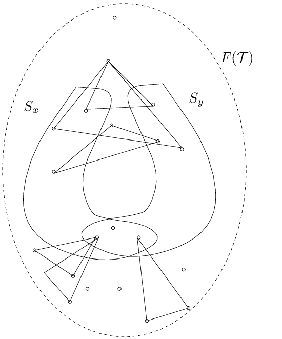
Now let the triple $\{a,b,c\}$ be in $T$; then $S_a\cup S_b\cup S_c=F(𝒯)$, $S_a\cap S_b=\mathrm{\varnothing }$, $S_a\cap S_c=\mathrm{\varnothing }$ and $S_b\cap S_c=\mathrm{\varnothing }$. We define

$$I_1=\{(x,y;z)\mid \{x,y,z\}\in T,x\in S_a,y\in S_b,z\in S_c\}.$$

It is easy to see that there is a one-to-one correspondence between the entries of $I_1$ and the triples of $T$ which maps $(x,y;z)\in I_1$ to $\{x,y,z\}\in T$. Moreover, $I_1$ forms one of the Latin interchanges into which we are decomposing the partial Latin square associated with $T$. Now the six conjugates of $I_1$ decompose $I$ into six disjoint Latin interchanges, where $ℐ=(I,I^{\prime })$ constitutes the Latin interchange and its disjoint mate corresponding to $𝒯=(T,T^{\prime })$.

However, the above condition of Lemma 7.2.8 is not necessary as is shown by the following example. The partial Steiner Latin squares corresponding to the trade $𝒯=(T,T^{\prime })$ where $T=\{136,148,159,239,246,257,$ $347,358\}$ and $T^{\prime }=\{139,158,146,259,236,247,357,348\}$ can be decomposed into six disjoint Latin interchanges. These may be obtained by taking the conjugates of the Latin interchange ${ℐ}_1=(I_1,I_1^{\prime })$, where $I_1=\{(1,3;6),(1,4;8),(1,5;9),(2,3;9),$ $(2,4;6),(2,5;7),(3,4;7),(3,5;8)\}$. This trade does not have the property set out in the above lemma but it is decomposable.

Thus to further our study we focus on the trades of volume less than ten.

REMARK: We note that if such a decomposition exists for each $i=1,\mathrm{\dots },6$ and each $x\in V$, the partial Latin square $I_i$ is such that $|R_x(I_i)|=|C_x(I_i)|=|E_x(I_i)|$ equals the replication number for symbol $x$. Also, since for $i=1,\mathrm{\dots },6$, it follows that $|T|=|I_i|$, the volume of each of the Latin interchanges ${ℐ}_i$ studied here is less than or equal to nine. In the paper [41] Keedwell classified the type of all Latin interchanges of volume less than or equal to 10. We have used his classifications when arguing that decomposition is not possible and in many of these cases we shall frequently use the following lemma.

Lemma 7.2.9

If the replication number of an element $e$ is $2$ or $3$, then for $i=1,\mathrm{\dots },6$ in any given Latin interchange ${ℐ}_i$, $e$ can only occur as a row or a column or a symbol. If the replication number of a symbol $e$ is $4$, then in any given Latin interchange ${ℐ}_i$, $e$ can only occur as a row, a column, or a symbol, or a row and a column, a row and a symbol, or a column and a symbol.

Proof.

Since a Latin interchange requires that $|R_e(I)|\ge 2$ and $|C_e(I)|\ge 2$, and $|E_e(I)|\ge 2$, when the replication number of $e$ is 2 or 3, the element cannot be split among all of rows and columns, or rows and symbols, or columns and symbols. Similarly when the replication number of $e$ is 4, the element cannot be split between rows, columns, and symbols.  

There are 25 Steiner trades of volume less than or equal to nine, and classifying these further we see that up to isomorphism there is one Steiner trade of volume 4, two Steiner trades of volume 6, two Steiner trades of volume 7, nine Steiner trades of volume 8 and eleven Steiner trades of volume 9. The triples of these trades are listed below. Our testing verified that for twelve of these Steiner trades the corresponding partial Steiner Latin square can be decomposed into six disjoint Latin interchanges satisfying the properties given in Question 7.1.4. These twelve cases are discussed below and the general nature of the decomposition is given. For the remainder of the cases, we present theoretical arguments that indicate why such a decomposition is not possible.

Trade of volume 4 ${𝒯}_0=(T,T^{\prime })$ where $T=\{123,156,435,426\}$ and $T^{\prime }=\{126,135,423,456\}$. This trade can be decomposed into Latin interchanges, corresponding to ${ℐ}_1=(I_1,I_1^{\prime })$ where $I_1$ = {(2, 3; 1),(5,6;1),(5,3;4),(2, 6; 4)}.

Trade of volume 6 ${𝒯}_1=(T,T^{\prime })$ where $T=\{123,145,167,247,346,357\}$ and $T^{\prime }=\{124,136,$ $157,237,345,467\}$. The replication numbers for the elements $1,\mathrm{\dots },7$ are:

Element	1	2	3	4	5	6	7
Replication number in $T$	3	2	3	3	2	2	3

Assume that the Latin interchanges associated with ${𝒯}_1$ can be decomposed into six disjoint Latin interchanges; then since $volume(T_1)=6$, one of these Latin interchanges must have type

$\left(\begin{array}{c}3+3\\ 3+3\\ 2+2+2\end{array}\right).$

So without loss of generality assume column $1$ contains three entries; but this implies there are three nonempty rows, which is a contradiction. Therefore no such decomposition exists.

Trade of volume 6 ${𝒯}_2=(T,T^{\prime })$ where $T=\{123,145,167,248,368,578\}$ and $T^{\prime }=\{124,136,157,$ $238,458,678\}$. This trade can be decomposed into Latin interchanges, corresponding to ${ℐ}_1=(I_1,I_1^{\prime })$ where $I_1=\{(1,3;2),(1,4;5),(1,7;6),(8,4;2),(8,3;6),(8,7;5)\}$.

Here we digress for a moment and use this trade to illustrate Lemma 7.2.8. Note that $S_1=S_8=\{1,8\}$, $S_2=S_5=S_6=\{2,5,6\}$ and $S_3=S_4=S_7=\{3,4,7\}.$

Trade of volume 7 ${𝒯}_3=(T,T^{\prime })$ where $T=\{123,145,167,246,257,356,347\}$ and $T^{\prime }=\{124,136,$ $157,237,256,345,467\}$. The only possible type of a Latin interchange $ℐ$ of volume seven is

$\left(\begin{array}{c}3+2+2\\ 3+2+2\\ 3+2+2\end{array}\right).$

Since the replication number of each element is $3$, this type is not possible.

Trade of volume 7 ${𝒯}_4=(T,T^{\prime })$ where $T=\{123,145,167,248,358,369,579\}$ and $T^{\prime }=\{124,136,$ $157,238,359,458,679\}$. A decomposition exists in which ${ℐ}_1=(I_1,I_1^{\prime })$ and where

$$I_1=\{(1,2;3),(1,5;4),(1,6;7),(8,2;4),(8,5;3),(9,6;3),(9,5;7)\}.$$

Trade of volume 8 ${𝒯}_5=(T,T^{\prime })$ where $T=\{123,145,167,248,257,346,378,568\}$ and $T^{\prime }=\{124,136,157,237,258,348,456,678\}$. As in the case of trade ${𝒯}_3$, the replication number for each element is 3, and so it is not possible to find a type

$\left(\begin{array}{c}W\\ X\\ Y\end{array}\right),$

in which the sums W, X, and Y consist only of 3s. Thus no decomposition exists.

Trade of volume 8 ${𝒯}_6=(T,T^{\prime })$ where $T=\{123,145,167,246,257,359,368,489\}$ and $T^{\prime }=\{124,136,157,235,267,389,459,468\}$. The replication numbers for the elements $1,\mathrm{\dots },9$ are as follows.

Element	1	2	3	4	5	6	7	8	9
Replication number in $T$	3	3	3	3	3	3	2	2	2

But there is no Latin interchange of size 8 which has type

$\left(\begin{array}{c}3+3+2\\ 3+3+2\\ 3+3+2\end{array}\right)$

and thus no decomposition exists.

Trade of volume 8 ${𝒯}_7=(T,T^{\prime })$ where $T=\{123,145,167,189,247,346,358,379\}$ and $T^{\prime }=\{124,136,158,179,237,345,389,467\}$. The replication numbers for the elements $1,\mathrm{\dots },9$ are as follows.

Element	1	2	3	4	5	6	7	8	9
Replication number in $T$	4	2	4	3	2	2	3	2	2

Assume that the Latin interchanges associated with ${𝒯}_7$ can be decomposed into six disjoint Latin interchanges; then since $volume(T)=8$, one of these Latin interchanges must have type

$\left(\begin{array}{c}3+3+2\\ X\\ Y\end{array}\right),$

where $X$ and $Y$ represent the appropriate sum values of the number of filled entries in the rows of the Latin interchange and the number of occurrences of each symbol in the Latin interchange. By Lemma 7.2.9, this implies that both row $4$ and row $7$ are simultaneously non-empty. Moreover, the elements $4$ and $7$ cannot occur as symbols. This is a contradiction as $247\in T$. Therefore no such decomposition exists.

Trade of volume 8 ${𝒯}_8=(T,T^{\prime })$ where $T=\{127,138,28A,379,459,46A,57A,689\}$ and $T^{\prime }=\{128,137,27A,389,45A,469,579,68A\}$. A decomposition exists in which ${ℐ}_1=(I_1,I_1^{\prime })$ where $I_1=\{(1,2;7),(1,3;8),(A,2;8),(9,3;7),(9,5;4),(A,6;4),(A,5;7),(9,6;8)\}$.

Trade of volume 8 ${𝒯}_9=(T,T^{\prime })$ where $T=\{123,145,167,189,24A,268,279,35A\}$ and $T^{\prime }=\{124,135,168,179,23A,267,289,45A\}$. A decomposition exists in which ${ℐ}_1=(I_1,I_1^{\prime })$ where $I_1=\{(1,2;3),(1,5;4),(1,6;7),(1,9;8),(A,2;4),(2,6;8),(2,9;7),(A,5;3)\}$.

Trade of volume 8 ${𝒯}_{10}=(T,T^{\prime })$ where $T=\{123,145,167,189,24A,35A,68A,79A\}$ and $T^{\prime }=\{124,135,168,179,23A,45A,67A,89A\}$. A decomposition exists in which ${ℐ}_1=(I_1,I_1^{\prime })$ where $I_1=\{(1,2;3),(1,5;4),(1,6;7),(1,9;8),(A,2;4),(A,5;3),(A,6;8),(A,9;7)\}$.

Trade of volume 8 ${𝒯}_{11}=(T,T^{\prime })$ where $T=\{123,145,167,189,24A,36A,58A,79A\}$ and $T^{\prime }=\{124,136,158,179,23A,45A,67A,89A\}$. A decomposition exists in which ${ℐ}_1=(I_1,I_1^{\prime })$ where $I_1=\{(1,2;3),(1,5;4),(1,6;7),(1,9;8),(A,2;4),(A,6;3),(A,5;8),(A,9;7)\}$.

Trade of volume 8 ${𝒯}_{12}=(T,T^{\prime })$ where $T=\{123,145,167,189,24A,68B,79B,35A\}$ and $T^{\prime }=\{124,135,168,179,23A,45A,67B,89B\}$. A decomposition exists in which ${ℐ}_1=(I_1,I_1^{\prime })$ where $I_1=\{(3,2;1),(4,5;1),(7,6;1),(8,9;1),(4,2;A),(8,6;B),(7,9;B),(3,5;A)\}$.

Trade of volume 8 ${𝒯}_{13}=(T,T^{\prime })$ where $T=\{123,145,24A,35A,678,69B,79C,8BC\}$ and $T^{\prime }=\{124,135,23A,45A,67A,68B,78C,9BC\}$. A decomposition exists in which ${ℐ}_1=(I_1,I_1^{\prime })$ where $I_1=\{(3,2;1),(4,5;1),(4,2;A),(3,5;A),(8,7;6),(9,B;6),(9,7;C),(8,B;C)\}$.

Trade of volume 9 ${𝒯}_{14}=(T,T^{\prime })$ where $T=\{145,167,189,239,257,268,346,358,479\}$ and $T^{\prime }=\{146,158,179,235,267,289,349,368,457\}$. Again the replication number for each element $e$ is 3. By Lemma 7.2.9, any Latin interchange $I_1$ must be a 3 $\times$ 3 subsquare. Assume that ${ℐ}_1$ is one of the Latin interchanges into which the partial Latin square associated with ${𝒯}_{14}$ can be decomposed. There are no 3 $\times$ 3 subsquares in the partial Latin square associated with $T$. We can show this by considering the partial Latin square $I_1$ containing the entry $(4,5;1)$. By Lemma 7.2.9, 4 can only occur as a row, and 1 can only occur as a symbol. Because $671\in T$, 6 must occur only as a row or column. Assume that 6 occurs only as a row. In this case, because $346\in T$, either $(6,4;3)$ or $(6,3;4)$ must occur in $I_1$ which is a contradiction since 4 can only be a row. Thus 6 must occur only as a column. In this case $(7,6;1)$ must be in $I_1$ and thus because $479\in T$, $(7,9;4)$ or $(7,4;9)$ must be an entry in $I_1$ which is a contradiction since we are assuming that 4 is a row. Thus no such decomposition exists.

Trade of volume 9 ${𝒯}_{15}=(T,T^{\prime })$ where $T=\{147,158,169,248,259,267,349,357,368\}$ and $T^{\prime }=\{148,159,167,249,257,268,347,358,369\}$. A decomposition exists where one Latin interchange is given by ${ℐ}_1=(I_1,I_1^{\prime })$ where $I_1=\{(1,4;7),(1,5;8),(1,6;9),(2,4;8),(2,5;9),$ $(2,6;7),(3,4;9),(3,5;7),$ $(3,6;8)\}$.

Trade of volume 9 ${𝒯}_{16}=(T,T^{\prime })$ where $T=\{123,145,167,189,248,257,269,346,479\}$ and $T^{\prime }=\{125,136,148,179,234,267,289,457,469\}$.

The replication numbers for the elements $1,\mathrm{\dots },9$ are as follows.

Element	1	2	3	4	5	6	7	8	9
Replication number in $T$	4	4	2	4	2	3	3	2	3

Assume $(6,9;2)\in I_1$, where $I_1$ forms one of the Latin interchanges into which we are decomposing the partial Latin square associated with $T$. Then by Lemma 7.2.9 we can say that 6 occurs only as a row, and 9 occurs only as a column. Since $167\in T$, then 7 occurs only as a column or symbol, and since $479\in T$, then 7 occurs only as a row or symbol. This means that 7 occurs only as a symbol. Thus $\{(6,1;7),(4,9;7)\}\subseteq I_1$. With this information, plus the fact that $257$ and $145$ are triples, we have four cases:

Case 1 $\{(5,2;7),(5,1;4)\}\subseteq I_1$. Since $(6,9;2)$, $(6,1;7)$ and $(4,9;7)$ are also in $I_1$, by Lemma 7.2.9 we find that $(6,3;4)$, $(1,3;2)$, $(1,9;8)$ and $(4,2;8)$ must be in $I_1$. Now it is easy to see that $I_1$ is not a Latin interchange. This is a contradiction.

Case 2 $\{(5,2;7),(5,4;1)\}\subseteq I_1$. Since $(6,9;2)$, $(6,1;7)$ and $(4,9;7)$ are also in $I_1$, by Lemma 7.2.9 we find that $(6,4;3)\in I_1$. Now either $(1,2;3)$ or $(2,1;3)$ must be in $I_1$. But both are impossible by Lemma 7.2.9. So this case is also impossible.

Case 3 $\{(2,5;7),(4,5;1)\}\subseteq I_1$. Since $(6,9;2)$, $(6,1;7)$ and $(4,9;7)$ are also in $I_1$, by Lemma 7.2.9 we find that $(8,9;1)$, $(8,4;2)$, $(6,4;3)$ and $(2,1;3)$ must be in $I_1$. Now it is easy to see that $I_1$ with these entries cannot be a Latin interchange. This is a contradiction.

Case 4 $\{(2,5;7),(1,5;4)\}\subseteq I_1$. Since $(6,9;2)$, $(6,1;7)$ and $(4,9;7)$ are also in $I_1$, by Lemma 7.2.9 we find that $(1,9;8)\in I_1$. Now either $(4,2;8)$ or $(2,4;8)$ must be in $T_1$. But both are impossible by Lemma 7.2.9.

Thus no decomposition exists.

Trade of volume 9 ${𝒯}_{17}=(T,T^{\prime })$ where $T=\{123,145,167,189,248,256,279,346,358\}$ and $T^{\prime }=\{124,136,158,179,235,267,289,348,456\}$.

The replication numbers for the elements $1,\mathrm{\dots },9$ are as follows.

Element	1	2	3	4	5	6	7	8	9
Replication number in $T$	4	4	3	3	3	3	2	3	2

Assume $(3,4;6)$ $\in I_1$, where $I_1$ forms one of the Latin interchanges into which we are decomposing the partial Latin square associated with $T$. Then by Lemma 7.2.9 we can say that 3 occurs only as a row, 4 occurs only as a column, and 6 occurs only as a symbol. Since $256\in T$, then 5 occurs only as a column or a row, and since $358\in T$, then 5 occurs only as a column or a symbol. This implies that 5 occurs only as a column. However, this leads to a contradiction since if we look at the triple $145$ of $T$, 4 and 5 must both occur as columns. Thus no decomposition exists.

Trade of volume 9 ${𝒯}_{18}=(T,T^{\prime })$ where $T=\{123,145,167,248,369,378,49A,579,68A\}$ and $T^{\prime }=\{124,136,157,238,379,459,48A,678,69A\}$.

The replication numbers for the elements $1,\mathrm{\dots },9,A$ are as follows.

Element	1	2	3	4	5	6	7	8	9	A
Replication number in $T$	3	2	3	3	2	3	3	3	3	2

Assume $(1,2;3)$ $\in I_1$, where $I_1$ forms one of the Latin interchanges into which we are decomposing the partial Latin square associated with $T$. Then by Lemma 7.2.9 we can say that 1 occurs only as a row, 2 occurs only as a column, and 3 occurs only as a symbol. Since $248\in T$, we see that 4 occurs only as a row or a symbol, and since $145$ is a triple, we see that 4 occurs only as a column or a symbol. Therefore, 4 occurs only as a symbol, 5 occurs only as a column, and 8 occurs only as a row. Since $49A\in T$, we see that 9 occurs only as a row or a column, and since $579\in T$, we see that 9 occurs only as a row or a symbol. Therefore, 9 occurs only as a row, A occurs only as a column, and 7 occurs only as a symbol. However, this leads to a contradiction since in the triple $378$ of $T$, 3 and 7 must both be symbols. Therefore no decomposition exists.

Trade of volume 9 ${𝒯}_{19}=(T,T^{\prime })$ where $T=\{123,145,167,189,24A,356,37A,468,479\}$ and $T^{\prime }=\{124,135,168,179,23A,367,456,489,47A\}$. A decomposition exists in which ${ℐ}_1=(I_1,I_1^{\prime })$ where $I_1=\{(1,2;3),(1,5;4),(6,7;1),(9,8;1),(A,2;4),(6,5;3),(A,7;3),(6,8;4),$ $(9,7;4)\}$.

Trade of volume 9 ${𝒯}_{20}=(T,T^{\prime })$ where $T=\{123,145,167,189,24A,368,39A,479,578\}$ and $T^{\prime }=\{124,136,158,179,23A,389,457,49A,678\}$.

The replication numbers for the elements $1,\mathrm{\dots },9,A$ are as follows.

Element	1	2	3	4	5	6	7	8	9	$A$
Replication number in $T$	4	2	3	3	2	2	3	3	3	2

Assume $(1,2;4)$ $\in I_1$, where $I_1$ forms one of the Latin interchanges into which we are decomposing the partial Latin square associated with $T$. Then, by Lemma 7.2.9, we can say that 2 occurs only as a column and 4 occurs only as a symbol. Since $23A\in T$, we see that $A$ occurs only as a row or a symbol, and since $49A\in T$, we find that $A$ occurs only as a row or a column. Therefore, $A$ occurs only as a row and we must have $(A,2;3),(A,9;4)\in I_1$. Then we must have $(8,9;3)\in I_1$. Since $678\in T$, we see that $6$ occurs only as a column or a symbol, and since $136\in T$, we find that $6$ occurs only as a row or a column. Therefore, $6$ occurs only as a column and we must have $(8,6;7),(1,6;3)\in I_1$. However, this leads to a contradiction since in the triple $457$ of $T$, 4 and 7 must both be symbols. Therefore no decomposition exists.

Trade of volume 9 ${𝒯}_{21}=(T,T^{\prime })$ where $T=\{123,145,167,189,24A,346,358,39A,479\}$ and $T^{\prime }=\{124,136,158,179,23A,345,389,467,49A\}$.

The replication numbers for the elements $1,\mathrm{\dots },9,A$ are as follows.

Element	1	2	3	4	5	6	7	8	9	$A$
Replication number in $T$	4	2	4	4	2	2	2	2	3	2

Assume that the partial Steiner Latin square $I$ associated with $T$ can be decomposed into six disjoint Latin interchanges; then, since $volume(T)=9$, one of these Latin interchanges must have type

$\left(\begin{array}{c}W\\ X\\ Y\end{array}\right),$

where $W$, $X$ and $Y$ are all odd and represent the appropriate sums for the number of symbols in each row and column and the frequency of each symbol’s occurrence in $I$, $|E_e(I)|$. However it is not possible to partition the multiset $\{4,2,4,4,2,2,2,2,3,2\}$ into three multisubsets such that the sum of the entries in each of these multisubsets is odd. Therefore no such decomposition exists.

Trade of volume 9 ${𝒯}_{22}=(T,T^{\prime })$ where $T=\{123,145,167,189,24A,36A,468,479,578\}$ and $T^{\prime }=\{124,136,158,179,23A,457,46A,489,678\}$.

The replication numbers for the elements $1,\mathrm{\dots },9,A$ are as follows.

Element	1	2	3	4	5	6	7	8	9	$A$
Replication number in $T$	4	2	2	4	2	3	3	3	2	2

Assume $(5,7;8)$ $\in I_1$, where $I_1$ forms one of the Latin interchanges into which we are decomposing the partial Latin square associated with $T$. Then, by Lemma 7.2.9, we can say that $5$ occurs only as a row, $7$ occurs only as a column, and $8$ occurs only as a symbol. On the other hand, since $167$ and $468$ are triples of $T$, we must have $(6,7;1),(6,4;8)\in I_1$. Now considering the triples $36A$ and $479$ of $T$, we have four different cases:

Case 1 $\{(6,3;A),(4,7;9)\}\subseteq I_1$ which means that 9 occurs only as a symbol by Lemma 7.2.9. Then $189$ being a triple of $T$ means that both 8 and 9 are symbols. This is a contradiction.

Case 2 $\{(6,3;A),(9,7;4)\}\subseteq I_1$ which means that 9 occurs only as a row, A occurs only as a symbol, and 3 occurs only as a column, by Lemma 7.2.9. Then $189$ being a triple of $T$ means that $(9,1;8)$ is a entry in $I_1$. Thus 1 occurs as both a column and a symbol. Since $123\in T$, this means that $(2,3;1)$ must be an entry in $I_1$, which means that 2 can only occur as a row. Then $24A$ being a triple of $T$ means that $(2,4;A)$ is an entry of $I_1$. Thus 4 occurs as both a column and a symbol. Then $145$ being a triple of $T$ means that $(5,1;4)$ must be an entry of $I_1$, since column 1 needs to have two entries in it. It is now easy to see that $I_1$ with these entries cannot be a Latin interchange. This is a contradiction.

Case 3 $\{(6,A;3),(4,7;9)\}\subseteq I_1$ which means that 9 occurs only as a symbol by Lemma 7.2.9, leading to a contradiction as in Case 1.

Case 4 $\{(6,A;3),(9,7;4)\}\subseteq I_1$ which means that 9 occurs only as a row, A occurs only as a column, and 3 occurs only as a symbol by Lemma 7.2.9. Then $189$ being a triple of $T$ means that that $(9,1;8)$ must be an entry in $I_1$. Thus 1 occurs as both a column and a symbol. Since $123\in T$, this means that $(2,1;3)$ must be an entry in $I_1$, which means that 2 can only occur as a row. Then $24A$ being a triple of $T$ means that $(2,A;4)$ must be an entry of $I_1$. Thus 4 occurs as both a column and a symbol. Then $145$ being a triple of $T$ means that $(5,4;1)$ must be an entry of $I_1$, since row 5 needs to have two symbols in it. It is now easy to see that $I_1$ with these entries cannot be a Latin interchange. This is a contradiction. Thus no decomposition is possible.

Trade of volume 9 ${𝒯}_{23}=(T,T^{\prime })$ where $T=\{123,145,167,248,368,49A,579,69B,8AB\}$ and $T^{\prime }=\{124,136,157,238,459,679,48A,68B,9AB\}$. A decomposition exists in which ${ℐ}_1=(I_1,I_1^{\prime })$ where $I_1=\{(3,2;1),(4,5;1),(7,6;1),(4,2;8),(3,6;8),(4,A;9),(7,5;9),(B,6;9),$ $(B,A;8)\}$.

Trade of volume 9 ${𝒯}_{24}=(T,T^{\prime })$ where $T=\{123,145,167,189,24A,36A,49B,58B,79A\}$ and $T^{\prime }=\{124,136,158,179,23A,45B,49A,67A,89B\}$. A decomposition exists in which ${ℐ}_1=(I_1,I_1^{\prime })$ where $I_1=\{(3,2;1),(4,5;1),(7,6;1),(8,9;1),(4,2;A),(3,6;A),(4,9;B),$ $(8,5;B),(7,9;A)\}$.

7.3 Conclusion

Thus in answer to Question 7.1.4, we have developed a theorem which determines the decomposability of certain Latin interchanges corresponding to Steiner minimal trades. Also, we have given a definite answer to the question of the decomposability of the Steiner partial Latin squares corresponding to each Steiner trade of volume less than or equal to 9.

Chapter 8 A census of critical sets in the Latin squares of order at most six

Many papers have examined the problems of determining the smallest and largest critical sets for particular orders of Latin square, or given examples of critical sets for small orders of Latin square. We give a brief overview of these papers.

The sizes of smallest critical sets for the Latin squares of orders four and five were determined in [29, 21]. Howse in [40] finds smallest critical sets for all the Latin squares of order six. This chapter enumerates all critical sets for each main class of order six, and Appendix Appendix 2 Critical sets in Latin squares of order 6 gives examples of each possible size of critical set in each main class.

Also, a paper [27] by Donovan gave examples of critical sets of order six of all possible sizes.

Adams and Khodkar in [4] give smallest critical sets for all the Latin squares of order at most seven. They also find, in [3], smallest weak and smallest totally weak critical sets for the Latin squares of order at most seven. The size of smallest strong critical sets in a Latin square has also been considered in the past (see [6]).

This chapter deals with critical sets of different sizes in the Latin squares of order at most six. First, for each main class of Latin square of order at most six, we calculate every possible critical set. These will be of various sizes. Then, for each main class of Latin square and possible size of critical set, we determine the main classes and isotopy classes for this set of critical sets. Next, we determine which of the main classes of critical sets are strong, near-strong, totally weak, and Bedford-Whitehouse totally weak. Some interesting properties concerning the greatest common divisors of numbers of critical sets across main classes in the $6\times 6$ Latin squares and ratios of various kinds are discussed.

Finally, for some of the Latin squares we consider, the possibility of the Latin square being partitioned into disjoint critical sets is examined.

8.1 Algorithms

To obtain the results presented here, we used two basic algorithms to calculate all critical sets of a given size $m$ for a given main class of $n\times n$ Latin squares.

The first was Algorithm 3.1.1, and the second algorithm used the improvements noted in Chapter 3. This algorithm divided the Latin square up into disjoint Latin interchanges, ensuring that each candidate for a critical set had at least one entry in each of the Latin interchanges.

For the case of the $6\times 6$ Latin squares, in the search for critical sets of size greater than 18, the improvements noted in Chapter 3 were used. We briefly recap these improvements here. For such subsets examined, the search speed was further increased by ensuring that no row or column was full and no symbol occurred six times. Such subsets cannot be critical sets since any entry may be removed from the relevant row, column or symbol set while maintaining the unique completion property.

We also use the result of Chapter 4, that lcs$(n)$ $\le n^2-3n+3$, to exclude from consideration any subset of size greater than 21.

8.2 Tables of results

8.2.1 Explanation of headings

The first column in the tables of results (Tables 8.1, 8.2, 8.3 and 8.4) is the main class number $n.z$ (LS), followed by the size(s) of the critical set(s) for the main class (Size), the number of critical sets of that size in the main class (#CS); this is then followed by the number of isotopy classes (#Iso) and the number of main classes of those critical sets (#Main). (The notation $n.z$ denotes main class $z$ in a Latin square of order $n$, as in the CRC Handbook of Combinatorial Designs, [16].)

For the next four columns, we consider representatives of each main class of critical sets, and list the number of critical sets of various “strengths” within the main classes of critical sets. That is, we calculate how many of the representatives of each main class of critical set have the various “strengths”. We need only consider representatives of each main class of critical set, since, for example, a strong critical set remains a strong critical set when the rows, columns and symbols are interchanged or swapped. Similarly, a near-strong critical set remains near-strong under permutations or interchanges of rows, columns or symbols. These last four columns are, in order, the number of near-strong critical sets (#NS), the number of strong critical sets (#Strong), the number of totally weak critical sets (#TW), and the number of Bedford-Whitehouse totally weak critical sets (#BWTW).

8.2.2 Latin squares of order 3

There is only one main class, denoted 3.1, for Latin squares of order three [16]:

1	2	3
2	3	1
3	1	2

3.1

For this Latin square, we have the results presented in Table 8.1 concerning the number of critical sets of every possible size.

Table 8.1: Critical set statistics for Latin squares of order 3

LS	Size	#CS	#Iso	#Main	#NS	#Strong	#TW	#BWTW
$3.1$	$2$	$9$	$1$	$1$	1	1	0	0
	$3$	18	$1$	$1$	1	1	0	0

8.2.3 Latin squares of order 4

There are two main classes, denoted 4.1 and 4.2, for Latin squares of order four [16]:

1 2 3 4 2 3 4 1 3 4 1 2 4 1 2 3			1 2 3 4 2 1 4 3 3 4 1 2 4 3 2 1
4.1			4.2

For these Latin squares, we have the results presented in Table 8.2 concerning the number of critical sets of every possible size.

Table 8.2: Critical set statistics for Latin squares of order 4

LS	Size	#CS	#Iso	#Main	#NS	#Strong	#TW	#BWTW
4.1	$4$	$32$	$1$	$1$	1	1	0	0
	$5$	$576$	$18$	$4$	4	4	0	0
	$6$	$128$	$4$	$2$	2	2	0	0
4.2	$5$	$96$	$1$	$1$	1	1	0	0
	$6$	$432$	$7$	$3$	3	3	0	0
	$7$	$48$	$1$	$1$	1	1	0	0

8.2.4 Latin squares of order 5

There are two main classes, denoted 5.1 and 5.2, for Latin squares of order five [16]:

1 2 3 4 5 2 3 4 5 1 3 4 5 1 2 4 5 1 2 3 5 1 2 3 4			1 2 3 4 5 2 1 4 5 3 3 4 5 1 2 4 5 2 3 1 5 3 1 2 4
5.1			5.2

For these Latin squares, we have the results presented in Table 8.3 concerning the number of critical sets of every possible size.

Table 8.3: Critical set statistics for Latin squares of order 5

LS	Size	#CS	#Iso	#Main	#NS	#Strong	#TW	#BWTW
$5.1$	$6$	$50$	$1$	$1$	1	1	0	0
	$7$	$1000$	$10$	$4$	4	4	0	0
	$8$	$30900$	$312$	$57$	57	57	0	0
	$9$	$18800$	$188$	$37$	37	37	0	0
	$10$	$2500$	$25$	$6$	6	6	0	0
$5.2$	$7$	$600$	$50$	$11$	10	10	1	1
	$8$	$21588$	$1802$	$322$	311	311	1	1
	$9$	$23718$	$1981$	$348$	348	348	0	0
	$10$	$2340$	$198$	$39$	38	36	2	0
	$11$	$216$	$18$	$4$	4	4	0	0

8.2.5 Latin squares of order 6

There are twelve main classes, denoted 6.1, …, 6.12, for Latin squares of order six [16]:

1 2 3 4 5 6 2 3 4 5 6 1 3 4 5 6 1 2 4 5 6 1 2 3 5 6 1 2 3 4 6 1 2 3 4 5	1 2 3 4 5 6 2 1 4 3 6 5 3 4 5 6 1 2 4 3 6 5 2 1 5 6 1 2 4 3 6 5 2 1 3 4	1 2 3 4 5 6 2 1 4 5 6 3 3 4 1 6 2 5 4 5 6 1 3 2 5 6 2 3 1 4 6 3 5 2 4 1	1 2 3 4 5 6 2 1 4 5 6 3 3 4 1 6 2 5 4 5 6 1 3 2 5 6 2 3 4 1 6 3 5 2 1 4
6.1	6.2	6.3	6.4

1 2 3 4 5 6 2 1 4 5 6 3 3 4 2 6 1 5 4 5 6 2 3 1 5 6 1 3 4 2 6 3 5 1 2 4	1 2 3 4 5 6 2 1 4 5 6 3 3 4 5 6 1 2 4 5 6 3 2 1 5 6 1 2 3 4 6 3 2 1 4 5	1 2 3 4 5 6 2 1 4 3 6 5 3 5 1 6 2 4 4 6 2 5 1 3 5 3 6 1 4 2 6 4 5 2 3 1	1 2 3 4 5 6 2 1 4 3 6 5 3 5 1 6 2 4 4 6 2 5 1 3 5 3 6 2 4 1 6 4 5 1 3 2
6.5	6.6	6.7	6.8

1 2 3 4 5 6 2 1 4 3 6 5 3 5 1 6 2 4 4 6 2 5 3 1 5 4 6 2 1 3 6 3 5 1 4 2	1 2 3 4 5 6 2 1 4 3 6 5 3 5 1 6 4 2 4 6 5 1 2 3 5 3 6 2 1 4 6 4 2 5 3 1	1 2 3 4 5 6 2 1 4 5 6 3 3 4 2 6 1 5 4 6 5 2 3 1 5 3 6 1 2 4 6 5 1 3 4 2	1 2 3 4 5 6 2 3 1 5 6 4 3 1 2 6 4 5 4 6 5 2 1 3 5 4 6 3 2 1 6 5 4 1 3 2
6.9	6.10	6.11	6.12

For these Latin squares, we have the results presented in Table 8.4 concerning the number of critical sets of every possible size.

Table 8.4: Critical set statistics for Latin squares of order 6

LS	Size	#CS	#Iso	#Main	#NS	#Strong	#TW	#BWTW
$6.1$	$9$	$72$	$1$	$1$	1	1	0	0
	$11$	$39384$	$547$	$97$	97	95	0	0
	$12$	$1161036$	$16149$	$2740$	2541	2513	11	8
	$13$	$3634344$	$50492$	$8481$	7815	7792	19	14
	$14$	$886428$	$12346$	$2090$	1931	1920	10	9
	$15$	$80064$	$1118$	$202$	182	168	8	0
	$16$	$3240$	$45$	$8$	8	8	0	0
	$17$	$108$	$3$	$1$	0	0	0	0
$6.2$	$11$	$7848$	$327$	$60$	50	48	3	3
	$12$	$658908$	$27477$	$4633$	4370	4325	35	27
	$13$	$3328908$	$138708$	$23267$	22226	22187	52	36
	$14$	$1800228$	$75035$	$12617$	12267	12263	11	8
	$15$	$192480$	$8022$	$1362$	1354	1351	3	1
	$16$	$15840$	$660$	$115$	113	113	0	0
	$17$	$240$	$10$	$3$	3	3	0	0
$6.3$	$11$	$1200$	$10$	$7$	2	2	0	0
	$12$	$192360$	$1603$	$836$	749	748	14	14
	$13$	$1837440$	$15315$	$7757$	7445	7440	33	29
	$14$	$1727880$	$14400$	$7279$	7252	7252	2	2
	$15$	$378928$	$3162$	$1610$	1610	1610	0	0
	$16$	$20280$	$169$	$90$	90	90	0	0
	$17$	$840$	$7$	$4$	4	4	0	0

Table 8.4 (continued) LS Size #CS #Iso #Main #NS #Strong #TW #BWTW $6.4$ $10$ $56$ $7$ $5$ 5 5 0 0 $11$ $34000$ $4250$ $2149$ 2001 1980 16 10 $12$ $1590608$ $198826$ $99654$ 94485 94024 197 136 $13$ $5498076$ $687262$ $344044$ 328754 327801 331 232 $14$ $1931424$ $241428$ $120895$ 116390 115691 58 34 $15$ $168752$ $21095$ $10586$ 10102 9704 137 10 $16$ $13736$ $1717$ $871$ 821 780 24 1 $17$ $148$ $19$ $11$ 9 9 1 1 $6.5$ $10$ $60$ $15$ $9$ 9 9 0 0 $11$ $42992$ $10748$ $5406$ 5132 5078 30 24 $12$ $1878236$ $469559$ $235063$ 224705 223776 401 292 $13$ $6475142$ $1618806$ $809952$ 778258 776251 648 473 $14$ $2182652$ $545663$ $273120$ 264790 263229 119 76 $15$ $192416$ $48104$ $24108$ 23304 22340 281 28 $16$ $16908$ $4227$ $2135$ 2041 1961 43 3 $17$ $112$ $28$ $16$ 15 15 0 0 $6.6$ $11$ $12888$ $358$ $187$ 177 175 0 0 $12$ $856908$ $23803$ $12005$ 11191 11155 64 55 $13$ $4097790$ $113839$ $57151$ 54038 53898 162 120 $14$ $1476864$ $41024$ $20664$ 19770 19697 27 23 $15$ $155196$ $4311$ $2201$ 2139 2117 8 4 $16$ $12744$ $354$ $186$ 175 166 3 0 $17$ $216$ $6$ $4$ 4 4 0 0

Table 8.4 (continued) LS Size #CS #Iso #Main #NS #Strong #TW #BWTW $6.7$ $12$ $4752$ $22$ $5$ 3 3 0 0 $13$ $212328$ $985$ $183$ 165 165 5 5 $14$ $893700$ $4151$ $736$ 706 705 3 2 $15$ $545508$ $2536$ $465$ 465 465 0 0 $16$ $125766$ $583$ $109$ 109 109 0 0 $17$ $8208$ $38$ $13$ 13 13 0 0 $18$ $648$ $3$ $1$ 1 1 0 0 $6.8$ $11$ $3264$ $408$ $75$ 67 66 3 2 $12$ $324608$ $40576$ $6817$ 6023 5986 37 33 $13$ $1826592$ $228335$ $38265$ 35161 35063 123 80 $14$ $1093796$ $136729$ $22909$ 21804 21764 10 8 $15$ $106296$ $13290$ $2260$ 2178 2155 10 1 $16$ $8464$ $1058$ $185$ 175 167 6 1 $17$ $216$ $27$ $5$ 5 5 0 0 $6.9$ $10$ $24$ $2$ $2$ 2 2 0 0 $11$ $13980$ $1165$ $596$ 546 535 7 7 $12$ $716352$ $59714$ $29939$ 27999 27723 127 84 $13$ $2784264$ $232027$ $116246$ 109378 108885 243 173 $14$ $1065876$ $88856$ $44575$ 42345 42068 24 19 $15$ $85884$ $7159$ $3607$ 3462 3314 72 4 $16$ $6960$ $580$ $302$ 283 259 15 1 $17$ $24$ $2$ $2$ 2 2 0 0

Table 8.4 (continued) LS Size #CS #Iso #Main #NS #Strong #TW #BWTW $6.10$ $10$ $4$ $1$ $1$ 1 1 0 0 $11$ $13748$ $3437$ $587$ 555 547 6 3 $12$ $858348$ $214587$ $35899$ 33814 33644 169 123 $13$ $3894038$ $973520$ $162538$ 154803 154404 279 195 $14$ $1715492$ $428873$ $71685$ 69560 69375 38 29 $15$ $155000$ $38753$ $6513$ 6355 6232 34 4 $16$ $10540$ $2635$ $461$ 443 423 13 1 $17$ $120$ $30$ $6$ 6 6 0 0 $6.11$ $10$ $40$ $10$ $3$ 3 3 0 0 $11$ $63540$ $15885$ $2673$ 2617 2590 9 5 $12$ $2292266$ $573254$ $95781$ 92453 92029 96 59 $13$ $7075888$ $1768972$ $295196$ 284917 284027 145 96 $14$ $2203696$ $550993$ $91977$ 88209 87499 39 22 $15$ $188344$ $47086$ $7890$ 7584 7175 161 8 $16$ $17172$ $4293$ $729$ 685 645 35 4 $17$ $36$ $9$ $2$ 1 1 0 0 $6.12$ $11$ $143208$ $1326$ $232$ 229 228 0 0 $12$ $3518478$ $32664$ $5510$ 5384 5358 7 6 $13$ $9025344$ $83568$ $14037$ 13636 13584 17 14 $14$ $2104704$ $19506$ $3315$ 3146 3107 6 4 $15$ $200340$ $1855$ $326$ 316 297 8 1 $16$ $17820$ $165$ $32$ 29 28 1 0

Dénes and Keedwell  [23] point out that, for a given order $n$, each isotopy class of $n\times n$ Latin squares has a number of Latin squares associated with it, and similarly each main class of $n\times n$ Latin squares has a number of isotopy classes associated with it. Similarly, for any given main class $n.z$ of $n\times n$ Latin squares and given size of critical set $m$, if we consider the main classes of critical sets of size $m$ within the main class $n.z$, we have several associated isotopy classes of critical sets. In the same way, if we consider the isotopy classes of critical sets of size $m$ within the main class $n.z$, we have several associated critical sets of size $m$ in the main class $n.z$.

In Tables 8.5 to 8.8, the head line refers to the twelve main classes of $6\times 6$ Latin squares, and the side line refers to the possible sizes of critical sets. For $6\times 6$ Latin squares, we consider results related to these observations.

Each isotopy class of critical sets in $6\times 6$ Latin squares has between 2 to 216 associated critical sets. This result is given in Table 8.5.

Table 8.5: Numbers of critical sets in each isotopy class of critical sets of order six

	$6.1$	$6.2$	$6.3$	$6.4$	$6.5$	$6.6$	$6.7$	$6.8$	$6.9$	$6.10$	$6.11$	$6.12$
9	72	-	-	-	-	-	-	-	-	-	-	-
10	-	-	-	8	4	-	-	-	12	4	4	-
11	72	24	120	8	4	36	-	8	12	4	4	108
12	12,36,72	8,12,24	8	8	4	36	216	8	6,12	4	2,4	54,108
13	36,72	12,24	60,120	4,8	2,4	18,36	108,216	4,8	6,12	2,4	4	108
14	36,72	12,24	60,120	8	4	36	108,216	4,8	6,12	4	2,4	54,108
15	36,72	12,24	24,40,120	4,8	4	36	108,216	4,8	6,12	2,4	4	108
16	72	24	120	8	4	36	54,216	8	12	4	4	108
17	36	24	120	4,8	4	36	216	8	12	4	4	-
18	-	-	-	-	-	-	216	-	-	-	-	-

Each main class of critical sets in $6\times 6$ Latin squares has either 1, 2, 3 or 6 associated isotopy classes of critical sets. This result is given in Table 8.6.

Table 8.6: Numbers of isotopy classes of critical sets in each main class of critical sets of order six

	$6.1$	$6.2$	$6.3$	$6.4$	$6.5$	$6.6$	$6.7$	$6.8$	$6.9$	$6.10$	$6.11$	$6.12$
9	1	-	-	-	-	-	-	-	-	-	-	-
10	-	-	-	1,2	1,2	-	-	-	1	1	1,3,6	-
11	1,3,6	3,6	1,2	1,2	1,2	1,2	-	3,6	1,2	2,3,6	1,2,3,6	3,6
12	1,2,3,6	1,2,3,6	1,2	1,2	1,2	1,2	1,3,6	1,2,3,6	1,2	1,2,3,6	1,2,3,6	1,2,3,6
13	2,3,6	1,2,3,6	1,2	1,2	1,2	1,2	1,3,6	1,2,3,6	1,2	1,2,3,6	1,2,3,6	3,6
14	1,2,3,6	1,2,3,6	1,2	1,2	1,2	1,2	1,2,3,6	1,2,3,6	1,2	2,3,6	2,3,6	3,6
15	1,2,3,6	1,2,3,6	1,2	1,2	1,2	1,2	1,3,6	3,6	1,2	1,2,3,6	1,3,6	1,2,3,6
16	3,6	3,6	1,2	1,2	1,2	1,2	1,3,6	2,3,6	1,2	1,2,3,6	3,6	3,6
17	3	1,3,6	1,2	1,2	1,2	1,2	1,3,6	3,6	1	3,6	3,6	-
18	-	-	-	-	-	-	3	-	-	-	-	-

8.3 Some observations

We define some notation used in the following observations. We shall denote the number of critical sets of size $x$ in a main class $n.z$ by $CS(n,z,x)$. The number of isotopy classes of critical sets of size $x$ in a main class $n.z$ shall be denoted $IC(n,z,x)$, and the number of main classes of these critical sets shall be denoted $MC(n,z,x)$. The greatest common divisor of the number of critical sets of all sizes in a particular main class $n.z$ will be referred to as GCDCS$(n,z)$.

We shall concentrate on observations concerning the $6\times 6$ Latin squares.

We find that when the main class $6.z$ is fixed and $x$ takes all possible values, $CS(6,z,x)$ / $IC(6,z,x)$ is in most cases close to an integer constant. There is one exception: the critical sets of size 17 in main class 6.1, where all other values of $CS(6,1,x)/IC(6,1,x)$ are approximately 72, but $CS(6,1,17)/IC(6,1,17)=36$. We also find that this integer constant is a multiple of GCDCS$(6,z)$. These ratios are given in Table 8.7, truncated at two decimal places. The last line tabulates the values of GCDCS$(6,z)$.

Table 8.7: Ratio of critical sets to isotopy classes of critical sets of order six

	$6.1$	$6.2$	$6.3$	$6.4$	$6.5$	$6.6$	$6.7$	$6.8$	$6.9$	$6.10$	$6.11$	$6.12$
9	72.00	-	-	-	-	-	-	-	-	-	-	-
10	-	-	-	8.00	4.00	-	-	-	12.00	4.00	4.00	-
11	72.00	24.00	120.00	8.00	4.00	36.00	-	8.00	12.00	4.00	4.00	108.00
12	71.89	23.98	120.00	8.00	4.00	36.00	216.00	8.00	11.99	4.00	3.99	107.71
13	71.97	23.99	119.97	7.99	3.99	35.99	215.56	7.99	11.99	3.99	4.00	108.00
14	71.79	23.99	119.99	8.00	4.00	36.00	215.29	7.99	11.99	4.00	3.99	107.90
15	71.61	23.99	119.83	7.99	4.00	36.00	215.10	7.99	11.99	3.99	4.00	108.00
16	72.00	24.00	120.00	8.00	4.00	36.00	215.72	8.00	12.00	4.00	4.00	108.00
17	36.00	24.00	120.00	7.78	4.00	36.00	216.00	8.00	12.00	4.00	4.00	-
18	-	-	-	-	-	-	216.00	-	-	-	-	-
gcd	36	12	2	4	2	18	54	4	12	2	2	54

In seven of the twelve main classes (6.1, 6.2, 6.7, 6.8, 6.10, 6.11, and 6.12), the ratio $MC(6,z,x)$/$IC(6,z,x)$ is close to 6 with a few exceptions. In the other five main classes (6.3, 6.4, 6.5, 6.6, and 6.9) this ratio is close to 2 with a few exceptions. These ratios are given in Table 8.8, truncated at two decimal places.

Table 8.8: Ratio of main classes of critical sets to isotopy classes of critical sets of order six

	$6.1$	$6.2$	$6.3$	$6.4$	$6.5$	$6.6$	$6.7$	$6.8$	$6.9$	$6.10$	$6.11$	$6.12$
9	1.00	-	-	-	-	-	-	-	-	-	-	-
10	-	-	-	1.40	1.66	-	-	-	1.00	1.00	3.33	-
11	5.63	5.45	1.42	1.97	1.98	1.91	-	5.44	1.95	5.85	5.94	5.71
12	5.89	5.93	1.91	1.99	1.99	1.98	4.40	5.95	1.99	5.97	5.98	5.92
13	5.95	5.96	1.97	1.99	1.99	1.99	5.38	5.96	1.99	5.98	5.99	5.95
14	5.90	5.94	1.97	1.99	1.99	1.98	5.63	5.96	1.99	5.98	5.99	5.88
15	5.53	5.88	1.96	1.99	1.99	1.95	5.45	5.88	1.98	5.95	5.96	5.69
16	5.62	5.73	1.87	1.97	1.97	1.90	5.34	5.71	1.92	5.71	5.88	5.15
17	3.00	3.33	1.75	1.72	1.75	1.50	2.92	5.40	1.00	5.00	4.50	-
18	-	-	-	-	-	-	3.00	-	-	-	-	-

In each main class $6.z$, GCDCS$(6,z)$ is a multiple of 2, and for those main classes with $3\times 3$ subsquares (6.1, 6.6, 6.7 and 6.12) this number is a multiple of 18.

We also note that in the main classes of the $4\times 4$ and $6\times 6$ Latin squares, the smallest and largest possible critical sets (4 and 7 for the $4\times 4$ case and 9 and 18 for the $6\times 6$ case) each have only one isotopy and main class.

This is an interesting property which we are unable to explain at the present time. It may be the case that the enumeration of all critical sets of order 7 would give more insight into this property.

8.4 Observations concerning the union of critical sets

For the $4\times 4$ and $6\times 6$ back-circulant Latin squares it is possible to find four disjoint critical sets which partition the corresponding Latin square. This can easily be generalised to the $n\times n$ case [2].

If $L$ is any $6\times 6$ Latin square it is possible to find three disjoint critical sets of size 12 which partition $L$. We give a visual representation of these decompositions for Latin squares from representatives of each of the main classes, denoted $6.1$, …, $6.12$.

$6.1$

$=$

1 1 2 1 2 3 6 1 2 3 6 5

$+$

5 6 2 5 6 3 4 5 4 6 4 1

$+$

1 2 3 4 3 4 6 5 5 2 3 4

$6.2$

$=$

1 3 5 1 2 3 6 5 2 6 2 4

$+$

2 4 6 4 3 4 5 2 1 3 5 3

$+$

1 3 5 2 6 5 6 4 1 6 4 1

$6.3$

$=$

6 1 3 1 2 5 1 5 2 6 2 4

$+$

2 4 6 5 3 5 4 3 6 1 3 1

$+$

1 3 5 2 4 6 4 6 2 4 3 5

$6.4$

$=$

1 3 5 1 2 1 3 4 6 6 3 5

$+$

3 6 2 6 6 4 4 5 2 3 1 4

$+$

1 2 4 5 4 3 5 6 2 5 1 2

$6.5$

$=$

1 3 5 1 2 6 3 5 3 6 5 4

$+$

3 5 6 2 4 6 4 5 6 2 1 2

$+$

1 2 4 4 6 3 5 2 1 1 4 3

$6.6$

$=$

6 1 3 1 1 2 3 5 2 6 2 4

$+$

2 3 4 6 3 4 5 6 4 5 4 1

$+$

1 5 2 4 5 2 6 6 1 3 3 5

$6.7$

$=$

6 1 6 5 1 2 4 2 5 3 4 3

$+$

2 4 5 2 3 5 6 3 4 1 6 1

$+$

1 3 4 3 6 4 5 1 6 2 5 2

$6.8$

$=$

1 3 5 1 2 4 4 6 3 6 3 2

$+$

3 4 5 2 6 5 2 3 5 1 4 1

$+$

1 2 6 4 3 6 5 1 2 4 6 5

$6.9$

$=$

1 3 5 1 2 4 6 2 4 1 3 6

$+$

4 5 6 2 3 5 5 1 6 3 5 4

$+$

1 2 3 4 6 6 4 3 5 2 1 2

$6.10$

$=$

1 3 5 1 2 1 3 5 6 6 4 3

$+$

3 4 6 2 5 6 4 2 1 4 2 5

$+$

1 2 5 4 6 3 4 6 5 3 2 1

$6.11$

$=$

1 3 1 5 6 2 3 1 2 4 6 5

$+$

4 5 6 2 6 2 4 5 3 6 3 4

$+$

1 2 3 4 5 3 4 6 1 5 1 2

$6.12$

$=$

1 5 1 2 6 3 4 2 3 6 4 5

$+$

3 5 6 2 3 6 4 4 1 6 1 3

$+$

1 2 4 4 3 5 5 6 2 5 1 2

Chapter 9 Conclusion

In this thesis, we have developed several new results. The algorithms developed in Chapter 3 have been used throughout the remainder of the thesis to discover new bounds and existence results on the sizes of possible critical sets.

We have proved a new bound on lcs$(n)$ in Chapter 4, and given many examples of critical sets of sizes not previously known.

In Chapter 5, a new bound was given on the maximum number of intercalates in Latin squares of orders $2^{\alpha }m$ and $2^{\alpha }m+1$ for $\alpha \ge 2$ and $m$ odd ($\alpha \ne 3$ in the $2^{\alpha }m+1$ case). Also, a critical set in Latin squares of order $4m$ was given, and large critical sets in intercalate-rich Latin squares of orders 11 and 14 were examined.

We have completed the spectrum of critical sets between the bounds conjectured by Nelder (${\displaystyle \frac{n^2}{4}}$ and ${\displaystyle \frac{n^2-n}{2}}$). This result was given in Chapter 6.

In Chapter 7, we looked at all trades of volume between 6 and 9, and determined which of the corresponding partial Steiner Latin squares were decomposable into disjoint Latin interchanges.

In Chapter 8, the new bound on lcs$(n)$ from Chapter 4 was used to reduce the search space of critical sets for Latin squares of order 6, and all the critical sets in Latin squares of order at most six were then determined.

Further research could include determining those values $s>{\displaystyle \frac{n^2-n}{2}}$ for which there exists a critical set of order $n$ and size $s$. Instead of looking at the maximum number of intercalates, we could look at the maximum number of $m\times m$ subsquares, $m>2$, in a Latin square of given order.

The questions proposed at the conclusion to Chapter 4 also deserve more research. That is, is there a relationship between critical sets of size lcs$(n)$ and Latin squares with $I(n)$ intercalates, and must critical sets with lcs$(n)$ entries have a missing row, column, and symbol?

Enumerating the critical sets for the Latin squares of order 7 is not possible with current computer hardware and algorithms, but may become possible in the future. This would settle the question of what lcs$(7)$ is, and could possibly provide more information to help prove new bounds on scs$(n)$. Such an enumeration might also give more information to assist in understanding the patterns noted in Chapter 8.

A further idea for research based on the results of Chapter 8 is to check the critical sets of size 17 and order 6 for a possible construction for a critical set of size ${\displaystyle \frac{n^2-n}{2}}+2$ for $n\ge 6$.

The results of this thesis could possibly also be used in music composition, as the 20th century composers Karlheinz Stockhausen [69] and Peter Maxwell Davies [36] have used Latin squares extensively in their compositions.

Appendix 1

Examples of critical sets

Here we give some examples of large critical sets for $n=5,7$, $9$, and $10$. By combining the results of the two papers  [31] and  [27], and this appendix, we can show the existence of critical sets of all sizes between $\lfloor {\displaystyle \frac{n^2}{4}}\rfloor$ and the current upper bound for lcs$(n)$ for $1\le n\le 10$.

A critical set of order 5 and size 11:

2 4 5 1 2 5 1 2 5 0 2 1

A critical set of order 7 and size 25:

0 3 2 7 5 3 5 4 7 6 6 5 4 3 2 4 3 5 4 7 2 6 3 6 3 7

A critical set of order 9 and size 40:

0 6 9 1 8 2 4 9 4 2 8 2 1 1 6 5 2 7 2 8 4 9 8 7 5 9 4 1 2 4 9 8 2 6 5 7 2 5 4 9 8

A critical set of order 9 and size 41:

0 7 1 3 8 4 1 4 3 1 9 5 9 1 7 6 8 4 5 8 4 9 1 6 6 3 1 3 9 1 8 6 5 7 1 5 6 7 3 4 9 8

A critical set of order 9 and size 42:

3 5 6 7 8 9 0 8 4 5 6 4 3 9 7 9 6 5 8 5 8 4 9 1 3 6 6 5 3 3 9 1 8 6 5 1 5 6 7 3 4 9 8

A critical set of order 9 and size 43:

3 9 0 4 6 1 9 8 6 7 9 8 4 6 1 3 2 9 8 3 2 1 8 9 4 2 1 6 1 3 7 9 8 2 9 8 7 4 6 2 1 8 7 9

A critical set of order 9 and size 44:

0 1 3 5 7 1 2 6 5 3 2 1 6 5 8 1 2 3 4 5 2 1 4 7 3 5 3 2 1 4 6 6 7 4 3 1 2 7 5 6 8 4 3 2 1

A critical set of order 10 and size 56:

0 1 4 3 6 5 8 7 10 9 4 1 5 6 8 3 1 8 7 5 6 1 3 9 4 5 1 10 4 3 8 5 3 10 1 4 6 7 6 9 1 5 3 10 6 7 3 4 5 1 9 8 5 4 6 3 1

A critical set of order 10 and size 57:

0 1 3 5 7 9 1 2 5 6 8 3 2 1 9 6 7 5 1 2 3 8 4 5 2 1 10 4 3 5 9 3 10 1 2 6 7 6 4 2 1 5 3 6 7 8 3 5 1 2 9 8 5 4 6 3 2 1

Appendix 2

Critical sets in Latin squares of order 6

This appendix is associated with Chapter 8 and gives examples of critical sets of all possible sizes in each of the 12 main classes, denoted 6.1 to 6.12, of $6\times 6$ Latin squares.

1 2 3 2 3 3 4 4 5	1 1 2 1 2 3 1 2 3 4 6	1 1 2 1 2 3 6 1 2 3 6 5	1 1 2 6 1 2 6 1 2 3 3 4 5
6.1, size 9	6.1, size 11	6.1, size 12	6.1, size 13

1 4 1 2 4 5 1 4 3 1 2 4 5 2	1 1 2 1 2 3 1 2 3 4 1 2 3 4 5	1 5 1 2 5 6 1 2 6 1 2 4 1 2 3 5	5 6 1 5 1 2 5 6 1 2 3 6 1 3 1 2 3
6.1, size 14	6.1, size 15	6.1, size 16	6.1, size 17

1 3 5 6 1 3 6 2 5 2 4	1 3 5 1 2 3 6 5 2 6 2 4	1 3 5 1 2 3 5 2 6 1 4 2 4	1 3 5 1 2 3 5 2 1 2 4 5 2 4
6.2, size 11	6.2, size 12	6.2, size 13	6.2, size 14

1 3 5 1 2 3 5 2 1 2 4 6 2 1 3	1 3 5 1 2 3 6 5 2 1 6 1 5 2 1 3	1 3 5 1 2 3 5 2 1 1 2 3 5 2 1 3 4	5 6 1 3 1 4 2 4 1 6 2
6.2, size 15	6.2, size 16	6.2, size 17	6.3, size 11

6 1 3 1 2 5 1 5 2 6 2 4	6 1 3 1 2 1 3 2 5 4 3 5 4	6 1 3 1 2 1 3 2 4 1 3 6 2 4	1 3 5 1 2 4 1 3 2 6 2 1 6 2 4
6.3, size 12	6.3, size 13	6.3, size 14	6.3, size 15

1 3 5 1 2 4 1 3 2 6 2 1 3 5 4 1	1 3 5 1 2 4 1 3 2 4 1 3 3 2 5 4 1	4 6 1 5 1 4 3 6 2 4	1 3 5 1 2 1 3 4 6 6 2
6.3, size 16	6.3, size 17	6.4, size 10	6.4, size 11

1 3 5 1 2 1 3 4 6 6 3 5	1 3 5 1 2 1 3 6 2 3 6 3 1	1 3 5 1 2 1 3 6 2 3 3 5 1 4	1 3 5 1 2 1 3 4 6 2 3 3 2 1 4
6.4, size 12	6.4, size 13	6.4, size 14	6.4, size 15

1 3 5 1 2 1 3 4 2 3 1 3 2 5 1 4	1 3 5 3 1 2 4 5 1 3 5 4 2 3 2 5 4	6 1 3 5 5 5 1 2 4 2	1 3 5 1 2 5 2 4 1 2 4
6.4, size 16	6.4, size 17	6.5, size 10	6.5, size 11

1 3 5 1 2 2 3 1 5 6 6 2	1 3 5 1 2 2 3 1 2 1 4 3 6	1 3 5 1 2 2 3 1 5 4 3 6 3 2	1 3 5 1 2 2 3 1 6 2 4 1 5 2 4
6.5, size 12	6.5, size 13	6.5, size 14	6.5, size 15

1 3 5 1 2 2 3 1 6 2 1 4 3 1 2 4	1 3 5 1 2 2 3 1 2 1 4 3 3 1 5 2 4	6 1 3 1 4 5 5 6 4 2 4	6 1 3 1 1 2 3 5 2 6 2 4
6.5, size 16	6.5, size 17	6.6, size 11	6.6, size 12

1 3 5 1 2 1 2 3 5 6 6 2 4	1 3 5 1 2 1 2 3 6 1 3 6 2 4	1 3 5 1 2 1 2 3 1 2 3 4 6 2 4	1 3 5 1 2 6 1 2 1 2 3 4 3 5 4 1
6.6, size 13	6.6, size 14	6.6, size 15	6.6, size 16

1 3 5 1 2 1 2 3 1 2 3 4 3 2 5 4 1	6 1 1 2 5 4 5 5 3 2 3 1	1 5 3 6 1 2 3 6 4 1 6 4 5	1 5 1 2 6 1 2 3 6 3 1 6 4 3
6.6, size 17	6.7, size 12	6.7, size 13	6.7, size 14

1 5 1 2 6 1 2 3 4 3 1 2 6 2 3	1 5 1 2 6 1 2 3 4 3 1 2 4 5 2 1	1 5 1 2 6 5 6 1 2 3 3 1 2 5 2 3 1	1 5 1 2 5 4 1 2 3 4 3 1 2 4 5 2 3 1
6.7, size 15	6.7, size 16	6.7, size 17	6.7, size 18

1 3 6 5 1 4 4 3 6 3 2	1 3 5 1 2 4 4 6 3 6 3 2	1 3 5 1 2 4 2 5 3 4 4 5 2	1 3 5 1 2 4 2 5 3 6 4 4 3 2
6.8, size 11	6.8, size 12	6.8, size 13	6.8, size 14

1 3 5 1 2 4 2 5 5 6 4 1 6 5 2	1 3 5 1 6 2 6 2 1 3 3 6 4 1 1 3	1 3 5 3 5 4 4 5 1 3 5 3 4 1 4 3 2	6 1 4 3 5 1 4 1 6 2
6.8, size 15	6.8, size 16	6.8, size 17	6.9, size 10

1 3 5 1 6 2 2 5 4 3 3	1 3 5 1 2 4 2 5 6 2 1 3	1 3 5 1 2 4 2 5 6 2 1 6 4	1 3 5 1 2 4 2 5 2 1 3 3 5 4
6.9, size 11	6.9, size 12	6.9, size 13	6.9, size 14

1 3 5 1 2 4 4 6 5 4 6 3 6 3 5	1 3 5 3 2 4 4 5 3 1 5 4 2 1 3 2	2 3 4 5 6 4 3 5 5 4 4 6 3 3 5 4 2	1 5 6 3 1 4 3 2 6 1
6.9, size 15	6.9, size 16	6.9, size 17	6.10, size 10

6 1 3 1 4 3 2 1 6 5 3	1 3 5 1 2 1 3 5 6 6 4 3	1 3 5 1 2 6 1 3 6 1 6 2 5	1 3 5 1 2 1 3 3 2 1 4 6 4 3
6.10, size 11	6.10, size 12	6.10, size 13	6.10, size 14

1 3 5 1 2 1 3 3 6 2 1 4 2 3 1	1 3 5 1 2 1 3 3 2 1 4 4 2 5 3 1	1 3 6 1 6 6 5 1 2 3 3 6 2 1 5 3 1	6 2 1 4 1 3 3 1 6 2
6.10, size 15	6.10, size 16	6.10, size 17	6.11, size 10

1 3 1 5 2 3 1 5 6 6 2	1 3 1 5 2 3 1 6 1 2 6 5	1 3 1 5 2 3 1 5 2 4 6 3 4	1 3 1 5 2 3 1 5 2 4 1 3 4 2
6.11, size 11	6.11, size 12	6.11, size 13	6.11, size 14

1 3 1 5 2 3 1 3 6 1 2 1 3 4 2	1 3 1 5 2 3 1 3 1 2 4 5 1 3 4 2	1 5 6 3 4 6 1 6 3 3 6 1 6 5 1 3 4	1 5 1 2 6 3 4 2 3 6 3
6.11, size 15	6.11, size 16	6.11, size 17	6.12, size 11

1 5 1 2 6 3 4 2 3 6 4 5	1 5 1 2 6 3 4 1 2 3 4 5 2	1 5 1 2 6 3 6 4 2 3 4 3 1 2	1 5 1 2 6 2 1 4 1 2 3 4 5 3 2
6.12, size 12	6.12, size 13	6.12, size 14	6.12, size 15

1 5 1 2 6 4 5 6 2 1 5 6 4 1 4 5

6.12, size 16

Appendix 3

Construction for Latin interchanges in a back-circulant array

This Appendix gives a construction for Latin interchanges referred to in Chapter 6, which are called “Variety 3” Latin interchanges there.

The construction given here is that of [31], and results in a Latin interchange $I$ in a back-circulant Latin square. Recall that the completion of the critical set $D$ given in Theorem 6.3.6 resulted in an $n\times n$ Latin square, denoted $ℒ𝒟$, of which the first ${\displaystyle \frac{n}{2}}$ rows were the same as an $n\times n$ back-circulant Latin square. $D$ contains entries from the first ${\displaystyle \frac{n}{2}}$ rows of $LD$, and the following result gives a Latin interchange $I$ which intersects $D$ in any given cell $(x,y)$ in those rows.

Let $𝒜$ denote the Latin subrectangle in $ℒ{𝒟}^{𝒯}$ (the transpose of $ℒ𝒟$) bounded by the entries $(x,y;y+x)$, $(n-1,y;y-1)$, $(x,{\displaystyle \frac{n}{2}}-1;{\displaystyle \frac{n}{2}}-1+x)$, and $(n-1,{\displaystyle \frac{n}{2}}-1;{\displaystyle \frac{n}{2}}-2)$. All future row and column references are relative to this subrectangle; that is, a reference to the entry $(i,j;k)$ means the entry $(i-x,j-y;k)$ in $ℒ{𝒟}^{𝒯}$.

Let $c={\displaystyle \frac{n}{2}}-y$, $r=n-x$, and $e=n+1-c$.

Define the sequence of numbers ${\alpha }_1,{\alpha }_2,\mathrm{\dots },{\alpha }_P$ to be integers where

${\alpha }_1$ $=$ $c-1(\mathrm{mod}e)\mathrm{and},\mathrm{for}i\ge 2,$

${\alpha }_i$ $=$ ${\alpha }_{i-1}(\mathrm{mod}(e-{\alpha }_1-\mathrm{\dots }-{\alpha }_{i-1})).$

Let $P$ be the value such that ${\alpha }_P\ne 0$ and ${\alpha }_{P+i}=0$ for all $i>0$. For $i=1,2,\mathrm{\dots },P$, let ${\delta }_i={\alpha }_1+{\alpha }_2+\mathrm{\dots }+{\alpha }_i$. Define

$A_0$ $=$ $\{(0,0;x+y),(0,c-1;c-1+x+y)\},\mathrm{and}\mathrm{if}{\alpha }_1\ne c-1\mathrm{define}$

$B_0$ $=$ $\{(c-1-ae,ae;c-1+x+y),(c-1-ae,(a+1)e;x+y)$

$\mid 0\le a\le {\displaystyle \frac{c-1-{\alpha }_1}{e}}-1\}.$

If ${\alpha }_1\ne 0$, define

$A_1$ $=$ $\{(e,c-1-{\alpha }_1;c-1+e-{\alpha }_1+x+y),(e,c-1;x+y)\},$

and if ${\alpha }_1\ne {\alpha }_2$ define

$B_1$ $=$ $\{({\alpha }_1-a(e-{\alpha }_1),c-1-{\alpha }_1;c-1+x+y),$

$({\alpha }_1-a(e-{\alpha }_1),c-1-{\alpha }_1+(a+1)(e-{\alpha }_1);c-1+e-{\alpha }_1+x+y)$

$\mid 0\le a\le {\displaystyle \frac{{\alpha }_1-{\alpha }_2}{e-{\alpha }_1}}-1\}.$

If $P\ge 2$, for $2\le i\le P$, define

$A_i$ $=$ $\{(e-{\delta }_{i-1},c-1-{\alpha }_i;c-1+e-{\delta }_i+x+y),$

$(e-{\delta }_{i-1},c-1;c-1+e-{\delta }_{i-1}+x+y)\}$

and if ${\alpha }_i\ne {\alpha }_{i+1}$, define

$B_i$ $=$ $\{({\alpha }_i-(e-{\delta }_i)a,c-1-{\alpha }_i+a(e-{\delta }_i);c-1+x+y),$

$({\alpha }_i-a(e-{\delta }_i),c-1-{\alpha }_i+(a+1)(e-{\delta }_i);c-1+e-{\delta }_i+x+y)\mid$

$0\le a\le {\displaystyle \frac{{\alpha }_i-{\alpha }_{i+1}}{e-{\delta }_i}}-1\}.$

Then the set $I=A_0\cup B_0\cup A_1\cup B_1\cup \mathrm{\dots }\cup A_P\cup B_P$ is the required Latin interchange.

Bibliography

- [1] P. Adams, R. Bean, and A. Khodkar. A census of critical sets in the latin squares of order at most six. Submitted for publication.
- [2] P. Adams, R. Bean, and A. Khodkar. Disjoint critical sets in latin squares. To appear in Congr. Numer.
- [3] Peter Adams and A. Khodkar. Smallest critical sets for the groups of size eight. J. Combin. Math. Combin. Comput., 32:23–32, 2000.
- [4] Peter Adams and A. Khodkar. Smallest critical sets for the Latin squares of orders six and seven. J. Combin. Math. Combin. Comput., 37:225–237, 2001.
- [5] R. A. Bailey, D. A. Preece, and P. J. Zemroch. Totally symmetric Latin squares and cubes. Util. Math., 14:161–170, 1978.
- [6] J. A. Bate and G. H. J. van Rees. The size of the smallest strong critical set in a Latin square. Ars Combin., 53:73–83, 1999.
- [7] R. W. Bean and E. S. Mahmoodian. On the size of the largest critical set in a latin square. To appear in Discrete Math.
- [8] Richard Bean and Diane Donovan. Closing a gap in the spectrum of critical sets. Australas. J. Combin., 22:199–210, 2000.
- [9] Richard Bean, Diane Donovan, Abdollah Khodkar, and Anne Penfold Street. Steiner trades that give rise to completely decomposable latin interchanges. In Proceedings of the Eleventh Australasian Workship on Combinatorial Algorithms, pages 17–30. School of Information Technology, University of Newcastle, 2000. To appear in the International Journal of Computer Mathematics.
- [10] David Bedford and David Whitehouse. Products of uniquely completable partial latin squares. Util. Math., 58:195–201, 2000.
- [11] L. Branković, P. Horák, M. Miller, and A. Rosa. Premature partial latin squares. Submitted for publication.
- [12] G. Carter, E. Dawson, and L. Nielsen. DESV: A latin square variation of DES. In Proceedings of the Workshop on Selected Areas in Cryptography, Ottawa, Canada, 1995, 1995.
- [13] Nicholas Cavenagh. The size of the smallest latin interchange in a back circulant latin square. Submitted for publication.
- [14] C. J. Colbourn, M. J. Colbourn, and D. R. Stinson. The computational complexity of recognizing critical sets. In Graph theory, Singapore 1983, pages 248–253. Springer, Berlin, 1984.
- [15] Charles J. Colbourn. The complexity of completing partial Latin squares. Discrete Appl. Math., 8(1):25–30, 1984.
- [16] Charles J. Colbourn and Jeffrey H. Dinitz. The CRC Handbook Of Combinatorial Designs. CRC Press, 1996.
- [17] J. A. Cooper, T. P. McDonough, and V. C. Mavron. Critical sets in nets and Latin squares. J. Statist. Plann. Inference, 41(2):241–256, 1994.
- [18] Joan Cooper, Diane Donovan, and Rebecca A. H. Gower. Critical sets in direct products of back circulant Latin squares. Util. Math., 50:127–162, 1996.
- [19] Joan Cooper, Diane Donovan, and Jennifer Seberry. Latin squares and critical sets of minimal size. Australas. J. Combin., 4:113–120, 1991.
- [20] Joan Cooper, Diane Donovan, and Jennifer Seberry. Secret sharing schemes arising from Latin squares. Bull. Inst. Combin. Appl., 12:33–43, 1994.
- [21] D. Curran and G. H. J. van Rees. Critical sets in Latin squares. In Proceedings of the Eighth Manitoba Conference on Numerical Mathematics and Computing (Univ. Manitoba, Winnipeg, Man., 1978), pages 165–168, Winnipeg, Man., 1979. Utilitas Math.
- [22] P. Danziger and E. Mendelsohn. Intercalates everywhere. In Geometry, Combinatorial designs and related structures (Spetses, 1996), pages 69–88. Cambridge Univ. Press, Cambridge, 1997.
- [23] Jozsef Dénes and Donald Keedwell. Latin squares and their applications. English Universities Press, 1974.
- [24] D. Donovan, A. Khodkar, and A. P. Street. On doubling and tripling constructions for defining sets. To appear in Graphs and Combinatorics.
- [25] D. Donovan, A. Khodkar, and A. P. Street. On minimal defining sets in AG(d,3). Submitted for publication.
- [26] Diane Donovan. Critical sets for families of Latin squares. Util. Math., 53:3–16, 1998.
- [27] Diane Donovan. Critical sets in Latin squares of order less than . J. Combin. Math. Combin. Comput., 29:223–240, 1999.
- [28] Diane Donovan and Joan Cooper. Critical sets in back circulant Latin squares. Aequationes Math., 52(1-2):157–179, 1996.
- [29] Diane Donovan, Joan Cooper, D. J. Nott, and Jennifer Seberry. Latin squares: critical sets and their lower bounds. Ars Combin., 39:33–48, 1995.
- [30] Diane Donovan and Adelle Howse. Critical sets for Latin squares of order . J. Combin. Math. Combin. Comput., 28:113–123, 1998. Papers in honour of Anne Penfold Street.
- [31] Diane Donovan and Adelle Howse. Towards the spectrum of critical sets. Australas. J. Combin., 21:107–130, 2000.
- [32] Diane Donovan, Adelle Howse, and Peter Adams. A discussion of Latin interchanges. J. Combin. Math. Combin. Comput., 23:161–182, 1997.
- [33] Chin-Mei Fu, Hung-Lin Fu, and Wen-Bin Liao. A new construction for a critical set in special Latin squares. Congr. Numer., 110:161–166, 1995.
- [34] Chin-Mei Fu, Hung-Lin Fu, and C. A. Rodger. The minimum size of critical sets in Latin squares. J. Statist. Plann. Inference, 62(2):333–337, 1997.
- [35] B. Ganter and H. Werner. Co-ordinatizing Steiner systems. Ann. Discrete Math., 7:3–24, 1980.
- [36] Paul Griffiths. Peter Maxwell Davies. Robson Books, 1981.
- [37] Michiel Hazewinkel, editor. Encyclopaedia of Mathematics. Dordrecht, 1987. Translation of the Soviet Mathematical Encyclopaedia.
- [38] Katherine Heinrich and W. D. Wallis. The maximum number of intercalates in a Latin square. In Combinatorial mathematics, VIII (Geelong, 1980), pages 221–233. Springer, Berlin, 1981.
- [39] Adelle Howse. Latin interchanges, critical sets and associated structures. PhD thesis, The University of Queensland, 1998.
- [40] Adelle Howse. Minimal critical sets for some small Latin squares. Australas. J. Combin., 17:275–288, 1998.
- [41] A. D. Keedwell. Critical sets and critical partial Latin squares. In Combinatorics, graph theory, algorithms and applications (Beijing, 1993), pages 111–123. World Sci. Publishing, River Edge, NJ, 1994.
- [42] A. D. Keedwell. Critical sets for Latin squares, graphs and block designs: a survey. Congr. Numer., 113:231–245, 1996. Festschrift for C. St. J. A. Nash-Williams.
- [43] A. D. Keedwell. A note on critical sets for the elementary abelian -group. Util. Math., 49:69–84, 1996.
- [44] A. D. Keedwell. Critical sets for orthogonal Latin squares of small order. Congr. Numer., 125:51–64, 1997.
- [45] A. D. Keedwell. What is the size of the smallest Latin square for which a weakly completable critical set of cells exists? Ars Combin., 51:97–104, 1999.
- [46] A. Khodkar, 1998. Private communication.
- [47] G. B. Khosrovshahi and H. R. Maimani. On - Steiner trades of small volumes. Ars Combin., 52:199–220, 1999.
- [48] A. Kotzig and J. Zaks. The three permutations theorem. Ars Combin., 16:113–117, 1983.
- [49] C. C. Lindner and C. A. Rodger. Design Theory. CRC Press, 1997.
- [50] E. S. Mahmoodian. Defining sets and uniqueness in graph colorings: a survey. J. Statist. Plann. Inference, 73(1-2):85–89, 1998. R. C. Bose Memorial Conference (Fort Collins, CO, 1995).
- [51] E. S. Mahmoodian and M. Mahdian. On the uniquely list colorable graphs. In Proceedings of the 28th Annual Iranian Mathematics Conference, Part 1 (Tabriz, 1997), pages 319–326. Tabriz Univ., Tabriz, 1997.
- [52] E. S. Mahmoodian, Reza Naserasr, and Manouchehr Zaker. Defining sets in vertex colorings of graphs and Latin rectangles. Discrete Math., 167/168:451–460, 1997.
- [53] E. S. Mahmoodian, Nasrin Soltankhah, and Anne Penfold Street. On defining sets of directed designs. Australas. J. Combin., 19:179–190, 1999.
- [54] E. S. Mahmoodian and G. H. J. van Rees. Critical sets in back circulant Latin rectangles. Australas. J. Combin., 16:45–50, 1997.
- [55] Brendan McKay, 1999. Private communication.
- [56] John Nelder. Critical sets in latin squares. CSIRO Division of Math. and Stats Newsletter, 38:4, 1977.
- [57] John Nelder, 1979. Private communication to Jennifer Seberry.
- [58] H. W. Norton. The squares. Ann. Eugenics, 9:269–307, 1939.
- [59] P. J. Owens and D. A. Preece. Complete sets of pairwise orthogonal Latin squares of order . J. Combin. Math. Combin. Comput., 18:83–96, 1995.
- [60] Donald Preece, 2000. Private communication.
- [61] Edward M. Reingold, Jurg Nievergelt, and Narsingh Deo. Combinatorial algorithms: theory and practice. Prentice-Hall Inc., Englewood Cliffs, N.J., 1977.
-
[62]
Glenn C. Rhoads.
http://remus.rutgers.edu/~rhoads/Code/lex_comb.c. - [63] Vladimir Nikolaevich Sachkov. Combinatorial Methods in Discrete Mathematics, 55 of Encyclopedia of mathematics and its applications. Cambridge University Press, 1996.
- [64] C. P. Schnorr and S. Vaudenay. Black box cryptanalysis of hash networks based on multipermutations. In Advances in cryptology—EUROCRYPT ’94 (Perugia), pages 47–57. Springer, Berlin, 1995.
- [65] Jennifer Seberry and Anne Penfold Street. Strongbox secured secret sharing schemes. Util. Math., 57:147–163, 2000.
- [66] Bohdan Smetaniuk. On the minimal critical set of a Latin square. Util. Math., 16:97–100, 1979.
- [67] D. R. Stinson and G. H. J. van Rees. Some large critical sets. Congr. Numer., 34:441–456, 1982.
- [68] Anne Penfold Street. Defining sets for -designs and critical sets for Latin squares. New Zealand J. Math., 21:133–144, 1992.
- [69] Richard Toop. Stockhausen’s Klavierstück VIII (1954). Miscellanea Musicologica, 10, 1979.